A Dynamic Cournot Model with Brownian Motion

Hyungho Youn¹, Victor J. Tremblay²

¹Seoul Institute, Seoul, Korea.
²Oregon State University, Corvallis, USA.

DOI: 10.4236/tel.[phone]                

Abstract

In this paper we develop a stochastic version of a dynamic Cournot model. The model is dynamic because firms are slow to adjust output in response to changes in their economic environment. The model is stochastic because management may make errors in identifying the best course of action in a dynamic setting. We capture these behavioral errors with Brownian motion. The model demonstrates that the limiting output level of the game is a random variable, rather than a constant that is found in the non-stochastic case. In addition, the limiting variance in firm output is smaller with more firms. Finally, the model predicts that firm failure is more likely in smaller markets and for firms that are smaller and less efficient at managing errors.

Keywords

Dynamic Cournot Model, Brownian Motion

1. Introduction

The starting point of oligopoly theory is the static Cournot model. It provides an example of Nash equilibrium and embeds a variety of possible market outcomes. One is the Cournot Limit Theorem, which states that the Cournot-Nash equilibrium is the monopoly outcome in a market with one firm, and approaches the competitive equilibrium as the number of competitors approaches infinity¹.

More sophisticated oligopoly models consider cases where firms interact over time. For example, in a Cournot-type supergame where the Cournot game is repeated in every period from now to eternity, an appropriately defined trigger strategy can support cooperation in every period (Friedman [3] ). Other models are dynamic because firms are slow to change their strategic variables, causing it to take time for firms to reach equilibrium. This can occur when change is costly, which forces firms into a differential oligopoly game. In cases such as these, the strategic variable (output or price) evolves to a limiting outcome that differs from the static Nash equilibrium that would occur if the change was instantaneous (i.e., the cost of change is zero). For example, Driskill and McCafferty [4] found that when output was slow to change in a Cournot-type game, the limiting output level fell between the static Cournot and perfectly competitive outcomes².

In this paper, our goal is to extend the dynamic Cournot model to include management errors. Brownian motion is used to model these behavioral errors. To our knowledge, we are the first to incorporate Brownian motion into an oligopoly model. By adding this stochastic component, we are able to show that output converges to a random variable rather than a constant, as in the deterministic dynamic Cournot model. In the stochastic model, the limiting variance in firm output is smaller in duopoly than in monopoly. Finally, the stochastic model predicts that firm failure is more likely in smaller markets and for firms that are smaller in size and are less efficient at coping with behavioral errors. These results provide us with a better understanding of stochastic markets, in particular the exit patterns of firms when managerial errors are present.

The remainder of the paper is organized as follows. In Section 2 we summarize the deterministic model on which our stochastic model is built. In Section 3 we develop the stochastic version of the dynamic Cournot model by adding Brownian motion. Here, we derive the limiting distribution of the game and investigate the consequences of allowing one firm to be superior at coping with errors. In Section 4 we analyze the effect of management error on firm failure. The final section provides a brief conclusion.

2. The Deterministic Dynamic Model

Our stochastic model builds from a deterministic dynamic model that we develop in this section. Several scholars have investigated a dynamic version of the Cournot model. For example, Maskin and Tirole [6] considered a duopoly model that is made dynamic by requiring firms to alternatively choose their levels of output. Driskill and McCafferty [4] and Dockner [7] modeled dynamics by introducing a cost of adjusting firm output over time. In models such as these, firms have dynamic best-reply functions, such that a firm’s best reply depends on its own and its rival’s past output decisions. An important conclusion of these models is that the subgame perfect Nash equilibrium is more competitive than the static Cournot equilibrium. Because our stochastic model builds from the deterministic case, we first discuss a dynamic version of the deterministic Cournot model.

Consider a market with two firms (1 and 2) that produce homogeneous goods. The inverse demand function at

time t is linear:, where p is price, is firm i’s output level, and a is a positive constant. Firm i’s total cost of production is quadratic:, where and b are positive con-

stants. In this model, firm inertia is motivated by the cost of changing its level of output. This adjustment cost is

, where k > 0 is the adjustment cost parameter. Costs are assumed to be sufficiently low so

that both firms participate in this dynamic version of the game. At t = 0, each firm’s goal is to choose a production plan to maximize its discounted stream of profits:

(1)

which is subject to the discount factor and the initial condition that the output of firm i in period 0 is.

Dockner [7] solves this problem using dynamic programming methods. He showed that the solution depends on a set of dynamic best-reply functions, which are linear differential equations that are assumed to take the following form:

(2)

(3)

Parameter m is a function of the parameters of the model and represents firm i’s long-run sales target in the absence of firm j (i.e., firm i’s monopoly output). Parameter m will increase with the size of the market. These functions capture the strategic dynamics of the model. The solution to this system is:

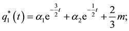(4)

(5)

where and are determined by the initial conditions [for i = 1 and 2]. Notice that as, a firm’s optimal level of output approaches, regardless of the initial output of the two firms.

3. A Dynamic Cournot Model with Brownian Motion

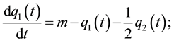
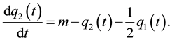
In this section we add a stochastic component to the dynamic Cournot model of the previous section. The stochastic component derives from a behavioral error that influences the dynamic best-reply functions of firms. One potential cause is the presence of boundedly rational managers who make errors when attempting to identify the best course of action in a dynamic setting³. Such errors may result from the cognitive limitations of managers coupled with the time pressure to make quick decisions. In our setup, behavioral errors occur when managers implement the dynamic best-reply functions and are captured by Brownian motion⁴. Adding Brownian motion (B_t) to the dynamic best-reply Equations (2) and (3) and converting them to stochastic difference equations produces:

(6)

(7)

Equations (6) and (7) describe each firm’s updating strategy in output, which is impacted by three forces. The first is m, which represents the firm’s sales target. Firm i’s output will increases when. The second force is rival output. As in the static Cournot model, firm i’s output falls with greater firm j output (i.e., and are strategic substitutes). The last term captures the effect of positive or negative behavioral management errors on firm output. The distribution of these errors is the same for both firms, but one firm may be better at dealing with these errors than the other firm. This occurs when firms have different Brownian motion parameters (i.e.,). Each parameter captures the magnitude of a firm’s behavioral error. For example, if managers do not make errors, then and the model collapse to the deterministic dynamic model. If behavioral errors exist and firm 1 is superior at coping with these errors, then.

Solving this system simultaneously produces a complex Gausian process, as described in Theorem 1.

Theorem 1: Given the game described above, the optimal paths of and are:

(8)

(9)

Proof: See Appendix.

If, then the difference in signs of the last set of terms in Equations (8) and (9) imply that.

In the limit, the solutions to Equations (8) and (9) require Ito integration. This result is described in the next theorem.

Theorem 2: Characteristics of the limiting distribution of Equations (8) and (9) as t → ∞ are:

(10)

(11)

A comparison of the pair of Equations (4) and (5) with the equations in Theorem 2 reveals that unlike the deterministic Cournot model, does not converge to a constant but is now a random variable. In the deter-

ministic case, the optimal output level of each firm converges to. With management error causing Brownian motion, the optimal level of output has a mean of. Even with this business disturbance, the

steady state equilibrium is the same on average as in the non-stochastic Cournot model. However, the stochastic model has a non-zero variance as seen in Equation (11). Another feature of the model is that the mean value in the model with Brownian motion does not depend on the initial positions of the two firms.

The final issue of interest is the effect of assuming that firm 1 is superior at dealing with behavior errors. One might expect that firm 1’s limiting distribution would have a smaller variance. This is not the case, however, as the interaction effects across firms, as described in Equations (6) and (7), cause their distributions to converge to the same limit as.

To further analyze the effect of firm ability to cope with behavioral errors, consider the case where firms are equally capable (i.e.,). When this occurs, the limiting variance of each firm in Equation (11) be-

comes. One can see that the interaction effects reduce the limiting variance, by comparing the duopoly results with the monopoly result. The mean value of firm output equals in monopoly and equals in

duopoly. With a single firm, the limiting variance in the single Orstein-Uhlenbeck mean-reverting equation

equals, compared to a value of in the duopoly case⁵. A firm’s variance is smaller with more firms.

4. Behavioral Errors and Firm Failure

Firm failure is common in a free market economy. For example, Dunn et al. [10] found that approximately 80 percent of firms exit the market within 10 years of entry. This suggests that management inexperience that leads to errors is a likely cause of firm exit. In this section, we use a dynamic Cournot model with Brownian motion that is caused by management error to explain the exit process.

Consider a setting with the following characteristics. Assume an emerging market where firms enter by initially producing below their long-run optimal levels of output⁶. Firms are asymmetric, and firm 1 has the initial

strategic advantage, such that. Firm exit occurs when; once a firm exits, it

cannot re-enter the market in a later period⁷. From Equations (8) and (9), we know that the optimal output path for firm 1 is greater than that of firm 2. This suggests that firm 2 is more likely to fail than firm 1. In order to

simplify the analysis and focus on the importance of starting values, we assume that.

With these assumptions and by defining firm 1 and 2’s respective exit periods as and, we are able to formally describes the probability that firm 2 will exit the market.

Theorem 3: If firm 1 starts out larger than firm 2 in period 0, then the probability that equals 1. That is, firm 2 always fails before firm 1.

Proof: See Appendix.

Although there is still a chance that firm 1 will fail, its probability of failure diminishes with the exit of firm 2. When firm 2 exits the market, Equation (6) shows that firm 1 will grow more rapidly toward its long-run optimum. This increase in size helps insulate firm 1 from failure.

The next question of interest is the precise probability that firm 2 will exit. Is this probability less than 1 [i.e.,] or will firm 2 exit with certainty as t → ∞ [i.e.,]? The following theorem answers this question.

Theorem 4: Let the difference in starting values be sufficiently small, such that. In this case, the probability of firm 2 exit as t → ∞ is less than 1:.

Proof: See Appendix.

In order to gain greater insight into the likelihood of firm 2 failure, we calculate the lower bound on this probability. This model produces the following result.

Theorem 5: The lower bound on the probability of firm 2 exit is. That is, .

Proof: See Appendix.

The lower bound is less than 1, and it falls as m and increase and as decreases. This has a reasonable economic interpretation: firm 2 is likely to have a better chance of survival when it is larger in size, operates in a larger market (i.e., as m increases), and is better able to deal with behavioral errors (i.e., as diminishes). The prediction that a larger firm is less likely to fail than the smaller firm is consistent with the empirical evidence found in Dunn et al. [10] for a cross section of USA industries and with the evidence of Tremblay and Tremblay [11] for the USA brewing industry.

5. Concluding Remarks

In this paper, we have extended the dynamic Cournot model to include behavioral errors on the part of management. The dynamic portion of the model follows the literature by assuming that firms face a cost of adjusting output. Thus, firms do not immediately adjust output to a new equilibrium after a behavioral error is made. Management error in this dynamic setting is modeled with Brownian motion. To our knowledge, we are the first to include Brownian motion in an oligopoly model.

The model produces several interesting results. First, Theorem 2 shows that the limiting output level is a random variable rather than a constant, as is found in the non-stochastic version of the dynamic Cournot model. It also indicates that the limiting variance in firm output is smaller in duopoly than in monopoly. Finally, Theorems 2 - 5 indicate that the probability of firm failure decreases for markets that are larger in size and for firms that are larger and more efficient at dealing with behavioral errors.

Acknowledgements

We would like to thank Roland Eisenhuth, Jenny Lin, Todd Pugatch, Carol Tremblay, Edward Waymire, Patrick De Leenheer and two anonymous referees for helpful comments on an earlier version of the paper.

Appendix

Proof of Theorem 1

We present this system of Equations (6) and (7) in matrix form:

(A1)

The eigenvalues of a and and the corresponding eigenvectors is and. It is worthy to note that the eigenvalues are negative. It makes the path of converges.

We diagonalize this SDE system using the eigenvectors.

Let, , and

Transforming yields the transformed coordinate of x. We need to transform x to solve SDE.

(A2)

(A3)

(A4)

The solution of this stochastic equations is:

(A5)

(A6)

where (or) is the initial value.

From, we recover:

(A7)

(A8)

where (or) is the initial quantity of firm 1 (or 2). Substituting, we have:

(A9)

(A10)

Because of, we can rewrite (A10) into:

(A11)

QED

Proof of Theorem 2

From (A9) and (A11), the mean is:

(A12)

(A13)

The variance of (A9) and (A11) is the same as below:

(A14)

Since, we reset (A14):

(A16)

(A17)

Accordingly,

(A18)

(A19)

QED

Proof of Theorem 3

We multiply both sides of (A9) and (A11) by:

(A20)

(A21)

Let and. Then, hitting time of is the same as that of and so it suffice to see hitting time of. We can rephrase (A20) and (A21):

(A22)

(A23)

We put them in differential form,

(A24)

(A25)

Since the drifting term of is larger than but diffusion terms are the same, , i.e., firm 2 always fails earlier than firm 1. QED

Proof of Theorem 4

Let and. Then, we reset (A25):

(A26)

Since, the drift term is positive, so.

QED

Proof of Theorem 5

We reset (A25):

(A27)

We have to find a function such that in order to know

. It is a challenge and so we seek for a possible exploration of a lower bound for the probability.

We change the drift of (A27) so that we can find an explicit value of the possibility of hitting zero. We suggest a new stochastic process with a larger drift term:

(A28)

Since the new stochastic process has a larger drift term, the possibility of hitting 0 is less than the possibility of hitting zero. Therefore, once we find the possibility of hitting 0, it becomes a lower bound for. Let.

(A29)

Then, is a martingale process. Let’s put a closed interval set for. We know . Let (or) be a stopping time for to exit the interval at 0 (or). Notice that when,. By optional stopping theorem (see Grimmett and Stirzaker [12] ),

(A30)

(A31)

A lower bound for business failure is.

QED

NOTES

¹A similar conclusion emerges in the Bertrand model when products are differentiated. For a more complete discussion, see Shy [1] (Chapter 6) and Tremblay and Tremblay [2] (Chapter 10).

²Other examples that use this framework include Fisher [5] , Maskin and Tirole [6] and Dockner [7] .

³For a detailed discussion of industrial organization models with bounded rationality, see Spiegler [8] and Tremblay and Tremblay [2] .

⁴Brownian motion is described by a Wiener process. It is related to a stochastic process, much like a standard normal distribution is related to random variables. A normal distribution arises as a limiting distribution for a suitable sequence of random variables, while a Brownian motion arises as a limiting distribution for a suitable sequence of stochastic processes. More specifically, a standard Brownian motion {W(t): t ≥ 0} is a stochastic process that has a continuous path, is stationary, and is independent over time where W(t) ~ N(0, t) "t ≥ 0. Brownian motion has been extensively in the fields of physics, biology, and finance, as discussed by Oksendal [9] .

⁵For Orstein-Uhlenbeck mean-reverting equation, , see Oksendal [9] .

⁶This assumption is reasonable if firms are cautious when entering a new market. In any case, the main results of this paper are the same when we assume that firms start out by producing more than their long-run equilibrium level of output.

⁷This can occur if firm exit tarnishes the reputation of the firm to such an extent that the cost of reentry is prohibitively high.

Conflicts of Interest

The authors declare no conflicts of interest.

References

[1]	Shy, O. (1995) Industrial Organization: Theory and Applications. MIT Press, Cambridge.
[2]	Tremblay, V.J. and Tremblay, C.H. (2012) New Perspectives on Industrial Organization: With Contributions from Behavioral Economics and Game Theory. Springer, Berlin. http://dx.doi.org/10.1007/978-1-4614-3241-8
[3]	Friedman, J.W. (1971) A Noncooperative Equilibrium for Supergames. Review of Economic Studies, 28, 1-12. http://dx.doi.org/10.2307/2296617
[4]	Driskill, R.A. and McCafferty, S. (1989) Dynamic Duopoly with Adjustment Costs: A Differential Game Approach. Journal of Economic Theory, 49, 324-338. http://dx.doi.org/10.1016/0022-0531(89)90085-9
[5]	Fisher, F. (1961) The Stability of Cournot Oligopoly Solutions: The Effects of Speeds of Adjustment and Increasing Marginal Costs. Review of Economic Studies, 28, 125-135. http://dx.doi.org/10.2307/2295710
[6]	Maskin, E. and Tirole, J. (1987) A Theory of Dynamic Oligopoly, III: Cournot Competition. European Economic Review, 31, 947-968. http://dx.doi.org/10.1016/0014-2921(87)90008-0
[7]	Dockner, E. (1992) A Dynamic Theory of Conjectural Variations. Journal of Industrial Economics, 11, 377-394. http://dx.doi.org/10.2307/2950530
[8]	Spiegler, R. (2011) Bounded Rationality and Industrial Organization. Oxford University Press, Oxford.
[9]	Oksendal, B. (2002) Stochastic Differential Equations: An Introduction with Applications. 5th Edition, Springer, Berlin.
[10]	Dunne, T., Roberts, M. and Samuelson, L. (1988) Patterns of Firm Entry and Exit in USA Manufacturing Industries. Rand Journal of Economics, 19, 495-515. http://dx.doi.org/10.2307/2555454
[11]	Tremblay, V.J. and Tremblay, C.H. (2005) The USA Brewing Industry: Data and Economic Analysis, MIT Press, Cambridge.
[12]	Grimmett, G.R. and Stirzaker, D.R. (2001) Probability and Random Processes. Oxford University Press, Oxford.