MICROMEGAS Signal: Numerical Simulation Based on Neon-Isobutane and Neon-DME ()
1. Introduction
MICROMEGAS [1] is a high gain gaseous detector, which can stand up alone without a need of an additional pre-amplification. It is a new gaseous detector initially developed for track-in high-rate, high-energy, physics experiments since 1990. It shows higher counting rate capacity up to 108 mm2∙s−1, position-sensitive with spatial resolution better than 100 microns and good performance of radiation hardness [2] [3] , which has been developed since 1996 at SACLAY, France [4] . MICROMEGAS is a Parallel Plate Detector (PPD) with three electrodes, cathode, micromesh and anode and a narrow amplification space, typically 50 - 100 microns, between the micromesh and the anode.
The detector gain depends directly on the distance between the micromesh and anode; therefore, controlling the geometry of the amplification region is crucial in order to achieve good energy resolution and excellent timing properties [5] . These results were confirmed by a similar structure having wider amplification gap and thicker metallic grid [6] .
2. MICROMEGAS Description and Operating
Detailed descriptions of MICROMEGAS are given in [1] [3] and [7] . A two-stage parallel plate avalanche chamber has a narrow amplification gap defined by the anode plane and a cathode plane made by Ni electroformed micromesh. Several 500 LPI, 5 × 5 cm2 and of micro-mesh pitch (pg) with a conversion gap of 3 mm, an amplification gap of 100 mm with a strip pitch of 317 mm, have been designed and fabricated. The parallelism between the micromesh grid and the anode is maintaining by spacers of 150 mm in diameter and placing every 2 mm. They are printedon a thin epoxy substrate by conventional lithography of a photo-resistive polyamide film. The thickness of the film defines the amplification gap. This cheap and simple process allows the construction of large detectors with excellent uniformity and energy resolution over the whole surface. Figure 1 shows geometric and physic descriptions of µ-MEGAS detector.
2.1. MCROMEGAS: Concept and Configuration
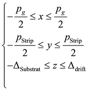
The geometry of MICROMEGAS detector is then, reproduced by form of cuboids Figure 2(b). The coordinate system used is showing in Figure 2(a), where:
![]()
Figure 1. MICROMEGAS description: physical & geometric processes.
![]() (a) (b)
(a) (b)![]() (c) (d)
(c) (d)
Figure 2. Coordinate system and geometric parameters (a) (b) and μ-mesh prototype (c) (d) used in MICROMEGAS detector.
 . (1)
. (1)
where pg is the Micro-Mesh pitch pstrip is the strip pitch.
2.2. Electric Field Configuration
The knowledge of the shape of the electric field lines close to the micromesh is a key issue for an optimal operation of the detector and especially for an efficient transfer of electrons to the amplification gap. The electric field is homogeneous in both the conversion and the amplification gap. It exhibits a funnel like shape around the openings of the micro-grid: field lines are highly compressed towards the middle of the openings, into a small pathway equal to a few microns in diameter. The compression factor is directly proportional to the ratio of the electric fields between the two gaps. Figure 3 displays details of the field lines near the grid used in the present test.
The electrons liberated in the conversion gap by the ionizing radiation follow these lines and are focused into the multiplication gap where amplification process takes place. The ratio between the Electric Field in the amplification gap and that in the conversion gap must be set at large values (>5) to permit a full electron transmission, and to reduce a part of ion cloud, produced in the avalanche, to escape into the conversion gap.
2.3. Electric Field and Potential Distributions
The mathematic term of potential is often calculated analytically using conformal transformations or Schwartz- Chritoffel transformation [7] . Our work is based on the use of Green functions [8] . The configuration that we want to study is presented in Figure 4.
After all calculus, considering all processes, we established the following form of Potential:
 (2)
(2)
![]()
Figure 3. Profile of the electric field lines close to the µ-Mesh in MICROMEGAS detector.
![]()
Figure 4. Configuring analytical calculation of the potential.
where  is the charge density in (y, z), and GD is the Dirichlet Function (Green Function) the weighting potential is presented in Figure 5.
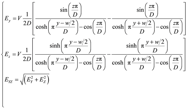
The weighing field is deduced from Equation (2)
 (3)
(3)
Equations (2) and (3) have been implemented in a MATLAB program; we treat different cases related to the geometric shapes of a track to determine the optimal width and pitch of the tracks. The results of the 3D potential and field distributions are shown in Figure 6 and Figure 7, respectively.
![]()
Figure 5. Weighting potential by applying 1 volt on a track (V = 1 V) and 0 volt on other.
![]()
Figure 6. 3D weighting potential distribution.
![]()
Figure 7. 3D weighting field distribution.
Note that the estimate of the potential distribution is insufficient to determine the optimal width of the tracks to get a good configuration MICROMEGAS detector. But it seems that the configurations (w1 = 280 microns, w2 = 317 microns and D) are satisfactory because the distributions are well presented. By against the corresponding distributions of the widths w = 100 µm tracks, have signal distortion (deformation) which causes instabilities and system disturbances.
The distributions of different configurations of weighting field are shown in the figure above. Note that the distributions of peaks increase with the growth of D. Moreover, the peaks of the first column of the field distribution (w = 100 microns) are very close, which produces overlaps (spark between the wire of the tracks). The remaining columns have peaks with a larger spacing. It is concluded that sufficient choice of track width minimizes system instability, as an example of the third column (w = 317 microns), which has only one peak band which further improves the stability; have good performance (better resolution) to MICROMEGAS.
3. Simulation Model
The analytical study of our system leads us to extract some equations that lead us to model our detector described above. The simulation model of the physical processes occurring within MICROMEGAS is based on the MATLAB Program that is the tool of simulation, and more effective for our work. In the general case, there are three types of parameters affecting the detector: the parameters related to the chamber (geometry), the gas parameters (diffusion, gain, mixing coefficients), the parameters of the trace (angle, energy, signal, type of particles). Figure 8 shows the principle operating and the simulator used for MICROMEGAS detector modeling.
3.1. Input Output Parameters Configuration and Characterization of MICROMEGAS
Table 1 shows some input output parameters used in the MICROMEGAS detector modeling.
3.2. Simulation of Charges Collected in MICROMEGAS
From Equation (4) [9] , [10] and Table 2 shown below [11] , we can estimate the charge collected Qi(t) (I = 1 to 5) in MICROMEGAS for different proportions of each gas mixture; using X-rays (5.9 keV) as a radiation source, the same program remains what we need to change the values of the coefficients Ai and Bi [11] - [13] . These parameters are adjusted by experience [14] .
 (4)
(4)
![]()
Figure 8. Principle operating and simulation tools used for MICROMEGAS detector.
![]()
Table 1. Input output parameters of micromegas detector.
![]()
Table 2. Mixing cefficients for different gas mixtures of an amplification gap d = 100 µm.
where Tw is the first Townsend Coefficient calculated in [12] , n0 is the electron number in Micro-Mesh.
The results are shown in Figure 9 and Figure 10.
First, we note that the temporal evolution of the total charge for both gas mixtures keeps the same evolution qualitatively. On the other hand, the charge decreases with the increase in the proportion of the quencher, and increases with the increase the electric field, in addition, the variation for Ne-isobutane is greater than that of Ne-DME. It is interesting to note that the total charge is simply the gain multiplied by the primary charge, and that in fact the amplified electrons do not contribute much to the final detected charge. The main contribution is clearly due to ions [15] . The proportion between the two contributions relates directly to the gain of the chamber. The fraction fe of the signal due to electrons is given by:
![]() (4a)
(4a)
![]()
![]() (a) (b)
(a) (b)
Figure 9. Charge in MICROMEGAS for different proportions of Ne-isobutane for Ea = 50 kV/ cm (a) and Ea = 80 kV/ cm (b).
![]()
![]() (a) (b)
(a) (b)
Figure 10. Charge in MICROMEGAS for different proportions of Ne-DME for Ea = 50 kV/ cm (a) and Ea = 80 kV/ cm (b).
Similarly, we can calculate the proportion of charge induced by ions:
![]() (4b)
(4b)
Qe is the charge induced by electron.
Simulation of the Electronic and Ionic Charge Fractions in MICROMEGAS
Table 2 and the Equations (4a) and (4b) allowed us dressed a Table 3, the results of charge fractions for two electric field configurations are presented in Figure 11.
From this figure, it is found that the fraction of charge induced by the electron for each gas mixing follows an exponential law; it decreases with increasing the amplification field and the proportion of the quencher. It tends to a minimum value (saturation) until the field is very intense. However, the proportion of charge induced by ions increases with increasing the field and the quencher, it tends to a limit value in higher field. The boundary value was:
![]()
Table 3. Induced charge fractions based in gas mixture.
![]()
![]() (a) (b)
(a) (b)
Figure 11. Induced charge fractions (fe) and (fion) based in Ne-isobutane (a) and Ne-DME (b).
![]() (4c)
(4c)
![]() (4d)
(4d)
4. Conclusions
The detector operating is the result of a detailed analysis of the physical phenomena. The calculus of the magnitudes characterizing this system (amplification, signal), depending on the thickness of the space, the gas mixture, geometrical configuration and the electrical distribution allowed amplification to determine the thickness of the space of the optimum gain, minimizing the effect of slight geometrical variations of the micro-grid. An amplification gap of 100 microns is optimal if it is desired to minimize the influence of the defects of planarity of the grid relative to the tracks. Simulations of μ-mega focused on the study of gas mixtures. To conduct this study, we used a 55Fe source emitting photons of 5.9 keV. For a gap width of 100 microns and a micro-grid prototype 500 LPI 5 × 5 cm2, based on Ne-isobutane and Ne-DME gas mixtures. In this study, we clarified the signal (Collected charge in MICROMEGAS). In MICROMEGAS, the avalanche starts much closer to the cathode due to the uniform electric field in the amplification gap. This property allows MICROMEGAS to obtain faster and more intense signals improving its performance (Spatial and temporal resolutions).
In conclusion, the good agreement between experimental measurements and simulation suggests that our simulation model is all the more satisfying. However, if there are disagreements. We are tempted to interpret these observed differences, as it is in any case of systematic uncertainties in the simulation, and physical phenomena occurring within the detector were not taken into account in our simulation program: as an example, the propagation of photons in the avalanche contributing to the extension of the lateral size of the avalanche, and the Pening effect, the discharge phenomenon, ..., these phenomena are taken into account as a perspective in the future work.
In brief, through the various comparisons between real data and simulated data, we achieved a better understanding of MICROMEGAS chambers by improving its performance.