An Analysis of the Jonsei and Purchase Prices in the Korean Housing Market ()
1. Introduction
The housing rental market in South Korea has a very unique form of housing rental contract called Jonsei, whose literal meaning is the “transfer rent”. The Jonsei is one of the most common housing rental contracts in South Korea and is not found elsewhere in the world. It has occupied a significant role in the rapid urbanization of the Korean economy. The Korean Government is attempting to stabilize the Jonsei price to improve housing security for the Korean people.
Rather than paying periodic rents for the right to use real property for a period of time, the tenant under the Jonsei contract transfers an up-front deposit, amounting usually up to 40% to 80% of the property value, to the landlord for the use of the property without making any periodic payments during the contract. When the contract matures, the tenant is entitled to get the full refund of the deposit in nominal terms with no interest. Thus, the implicit “rents” are paid by the tenant to the landlord in the form of the foregone returns from investing the lump sum deposit during the contract periods1. The Jonsei system eliminates the likelihood of tenant’s default on monthly rent as the deposit is maximized until the end of the contract period. However, the lump-sum deposit imposes a huge burden for younger renters and new households. The Jonsei system is crucial factor to achieving an in-depth understanding of the Korean housing market2.
The housing finance system Jonsei has been widely spread in South Korea, with the rapid urbanization for the last few decades. Especially, in 2000, only 41% of the households in Seoul owned their dwelling, 40% of them under Jonsei housing and 16% was monthly rent housing. In urban areas, Jonsei housing often corresponds to 2/3’s of all housing. The housing system Jonsei works in a way that effectively allows owners to leverage their investments by pulling out significant deposits which are used to purchase additional properties. It also allows owners to skirt government rental price controls and ownership restrictions.
Figure 1 depicts the movements in the JPR (Jonsei-to-Purchase price ratio). Evidently, the JPR has shown long swings: the ratio has steadily increased over the 1987-2002 period, followed by a decreasing trend until the late 2008. Another upward trend is observed in the recent period since then. The increase in the JPR can be interpreted in two ways. First, it can be interpreted that the increase of the JPR is simply a trend change. While the ratio stayed around average 37% - 40% until 1991, we can see the trend increase since the mid 1992. At that time, the expectation of house purchase price increase was continuously shrinking and fell short of the increase of Jonsei price, which brought out that the JPR showed long term upward trend. Consequently, the rapid increase of the JPR since late 1998 and 2008 may be interpreted as this kind of trend change.
However, we can also view the increase of the JPR as a signal for the future increase in house purchase price. The increase of the ratio is a phenomenon caused by faster increase of Jonsei price compared with house purchase price. Since the increase in Jonsei price means the increase of rental price, it can be predicted that the house price will be raised as the reflection of the rental price increase. In other words, as a result of the observation that house price does not reflect immediately the increase of Jonsei price, the JPR is increased, which can be interpreted that the house price will be increased in the future for adjustment. In reality, looking back past experiences, this kind of inference has its own validity since it has been shown that the increase rate in Jonsei price foreruns the increase rate in house purchase price3. Consequently, the former is an interpretation that the increase of the JPR is trend change accompanied by the expected increase rate of house price. The latter is an interpretation to be transitory change to be shown as a consequence of the meaning that the real price of house price does not reflect the intrinsic price immediately.
How the increase of the JPR is interpreted gives totally different meaning to investor and policy maker. If it is interpreted as the former, it is not necessary for investor and policy maker to put the significant meaning in the increase of the JPR. However, if it is interpreted as the latter, investor will have the opportunity to have arbitrage profit and policy maker has to prepare policy tools for the stability of house price. But, we don’t know ex ante
whether the increase of the JPR is caused by trend change or transitory change. In reality, even though the increase of the JPR is influenced by both changes, we don’t know which factor is stronger.
In this paper, we try to separate the trend and transitory change which are mixed in the change of the JPR. Through this separation, we answer the following questions: a) How much the degree of trend variation and that of cyclical variation are in the middle of the increase of the JPR? b) How cyclical variation is used as the pre- index for the future change in house purchase price? Using the state-space model, we try to separate the JPR as the trend component which shows the movement of intrinsic value and the cyclical component which appears in the process of real value’s reflecting the change of the intrinsic value. In the following section, the model is discussed briefly. In section 3, we present our empirical results. Section 4 concludes the paper with a few findings.
2. The Model
2.1. Theoretical Background
We present two possible interpretations of the changes in the JPR. The intrinsic value of house can be described as the following4:
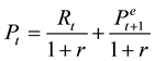 (1)
(1)
where  is the intrinsic price of house in period t,
  rent revenue at the end of period t,
  discount rate, and
  the house price predicted in period
  based on the information in period t. Here, we denote that the Jonsei price in period t is
 . It is assumed that the conversion rate of monthly rent to be used as the Jonsei is changed into monthly rent is the same with the discount rate. Then we get
 . Plugging this relation into (1), we can get
 (2)
(2)
Since the above equation means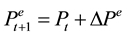 , where
  is the increase of house price expected in the next period, we can get


 (3)
(3)
Dividing both sides of the (3) by ,
,
![]() (4)
(4)
If![]() , where
, where ![]() is the expected increase rate of house price forecasted in period t with all available information, (4) will be
is the expected increase rate of house price forecasted in period t with all available information, (4) will be
![]() (5)
(5)
If there is no difference between the intrinsic value and actual price ![]() of house, we get
of house, we get![]() , which means that the JPR
, which means that the JPR ![]() depends on the expected increase rate of house price
depends on the expected increase rate of house price ![]() and discount rate
and discount rate
![]() . That the JPR is increasing means that the expected increase rate of house price was dropped down or the discount rate was raised up. However, if the real price of house does not reflect the intrinsic value of house well,
. That the JPR is increasing means that the expected increase rate of house price was dropped down or the discount rate was raised up. However, if the real price of house does not reflect the intrinsic value of house well,
there can be some change in the JPR ![]() without the change in the expected increase rate of house price
without the change in the expected increase rate of house price ![]() or discount rate
or discount rate![]() . For example, in spite of the increase in the intrinsic value of house
. For example, in spite of the increase in the intrinsic value of house ![]() caused by the increase in Jonsei price, if the actual price
caused by the increase in Jonsei price, if the actual price ![]() does not reflect this causality, the JPR
does not reflect this causality, the JPR ![]() will be increased without the change in the expected increase rate of house price
will be increased without the change in the expected increase rate of house price ![]() and discount rate
and discount rate![]() . In this case, the JPR
. In this case, the JPR ![]() will be decreased again, if the actual price
will be decreased again, if the actual price ![]() reflects the intrinsic value of house price
reflects the intrinsic value of house price
![]() . The discussion above allows us to interpret the change in the JPR in two ways. First, the change in the JPR means that there is some change in the expected increase rate of house price
. The discussion above allows us to interpret the change in the JPR in two ways. First, the change in the JPR means that there is some change in the expected increase rate of house price ![]() or discount rate
or discount rate![]() . Second, the change in the JPR is a kind of phenomenon caused by the situation in which the real price of house does not reflect the change in the intrinsic value of house well. This can be regarded as a kind of pre-index which forecasts the change in the future house price.
. Second, the change in the JPR is a kind of phenomenon caused by the situation in which the real price of house does not reflect the change in the intrinsic value of house well. This can be regarded as a kind of pre-index which forecasts the change in the future house price.
There are two reasons why the JPR is continuously increasing since the late of 1998 and 2008. The first is some change in the expected increase rate of house price ![]() or discount rate. The second is the change
or discount rate. The second is the change
which is appearing in the process of the actual house price reflecting the change in the intrinsic value of house. The change in the JPR caused by change in the expected increase rate of house price or discount rate is a kind of structural or trend change which is not changing easily in the short run. Of course, even though there is possibility that the discount rate influenced by market interest rate is easily changeable in the short run, the discount rate is affected by the long run interest rate rather than the short run interest rate because the transaction of real estate such as the house is accompanied by high cost. In general, considering that the long term interest rate is stable, it can be regarded that the discount rate is also not easily changeable in the short term.
Meanwhile, the change of the JPR can be a kind of cyclical variation which is shown in the process of the real price of house reflecting the intrinsic value of house. In other words, it can be regarded as short term change which is fluctuating in the center of intrinsic value during the adjustment of real price to the intrinsic value. Consequently, the work to separate the change of the JPR into the part of the change of intrinsic value of house and the part of the process of adjustment of real value into intrinsic value can be regarded as the job to separate the change of the ratio into trend and cyclical components. Since the two components are not observed, however, to separate the change of the ratio into two components is very difficult. With the data of the expected increase rate of house price, we can separate the part of intrinsic value out of the JPR. Unfortunately, however, the expected increase rate is not observed. Owing to this difficulty, we use unobserved component model with the use of State-Space Model. The statistical treatment is by the state space form and hence data irregularities such as missing observations are easily handled. Structural time series models can be formulated in terms of unobserved components, such as trends and cycles, that have a direct interpretation. Thus, they are designed to focus on the salient features of the series and to project these into the future and also provide a way of weighting the observations for signal extraction, so providing a description of the series.
2.2. Empirical Model
We set off with the decomposition of the JPR ![]() into two unobserved components:
into two unobserved components:
![]() (6)
(6)
where ![]() and
and ![]() are the trend (or permanent) and the cyclical (or transitory) component, respectively.
are the trend (or permanent) and the cyclical (or transitory) component, respectively.
The cyclical component is assumed to follow a stationary AR (2) process, with possible regime shifts (or asymmetric deviations) in its intercept, in the spirit of Friedman ( [5] [6] ) and Kim and Nelson [7] :
![]() (7a)
(7a)
![]() (7b)
(7b)
![]() (7c)
(7c)
![]() (7d)
(7d)
where ![]() is a discrete asymmetric shock dependent upon an unobserved state variable
is a discrete asymmetric shock dependent upon an unobserved state variable![]() , and
, and ![]() is a symmetric continuous shock.
is a symmetric continuous shock. ![]() is an indicator variable that determines the nature of the shocks to the economy. During the periods with
is an indicator variable that determines the nature of the shocks to the economy. During the periods with ![]() (and thus
(and thus![]() ), the JPR fluctuates around its trend level because the expectation (conditional on
), the JPR fluctuates around its trend level because the expectation (conditional on![]() ) of
) of ![]() is 0. During the other times with
is 0. During the other times with![]() , the JPR abruptly deviates from the trend via the term
, the JPR abruptly deviates from the trend via the term![]() . In Equations (7c), the variance of the symmetric disturbance
. In Equations (7c), the variance of the symmetric disturbance ![]() is allowed to be heteroskedastic across the two states of the housing market.
is allowed to be heteroskedastic across the two states of the housing market.
The trend component ![]() is assumed to be a generalized random walk with a regime-dependent drift and variances:
is assumed to be a generalized random walk with a regime-dependent drift and variances:
![]() (8a)
(8a)
![]() (8b)
(8b)
![]() (8c)
(8c)
where (8a) assumes that the trend component of the JPR follows a stationary AR(1) in its differences. In (8b), the drift term ![]() is subject to abrupt shift in the spirit of Hamilton [8] . We allow the variance of the shock
is subject to abrupt shift in the spirit of Hamilton [8] . We allow the variance of the shock ![]() to the trend to be state-dependent, as shown in Equations (8c)5.
to the trend to be state-dependent, as shown in Equations (8c)5.
To complete the model, we need to specify the evolution of the state variable![]() . To account for a persistence of normal and recession periods, we assume that
. To account for a persistence of normal and recession periods, we assume that ![]() evolves according to an exogenous first-order Markov-switching process:
evolves according to an exogenous first-order Markov-switching process:
![]() (9)
(9)
We cast the model described above comprising Equations (6) to (9) into a state-space form. The parameters of the resulting state space form are then estimated via the approximate maximum likelihood algorithm. Using the estimated parameters of the model, the estimates of the probabilities of the two regimes and the two components are constructed as well. We will discuss the estimation results in the following section
3. Empirical Analysis
The original data used in this paper are the seasonally adjusted nationwide housing purchase price index and Jonsei price index over January 1987 to September 2011, compiled and published by the Kookmin bank. The original indices are available in monthly frequency, but we use their quarterly average to facilitate the estimation6. We then rescale the ratio of the Jonsei and purchase price indices, so that the rescaled ratio matches the actual ratio which has been officially compiled since June 2011.
Before estimating the model parameters, we run unit root tests for the JPR series. These tests also constitute a specification test for the model, since the specification in Equations (6) and (8a) is only valid when the JPR series has a stochastic trend. The results of the Augmented Dickey-Fuller (ADF) and Phillips-Perron (PP) tests support that the JPR series is differently stationary. We then estimate the model from the Section 2, and report the results in Table 1.
We first discuss the results for the trend component, whose mean and variances are clearly regime dependent. In regime 1 with ![]() the drift term
the drift term ![]() takes
takes![]() , which is statistically insignificant. In regime 2 with
, which is statistically insignificant. In regime 2 with ![]() however, the drift term is significantly positive
however, the drift term is significantly positive![]() . The disturbance to the trend component is also regime dependent, exhibiting much lower volatility in regime 2. The combined results for the drift and variances imply that the regime 2 is where the JPR increases persistently around the stochastic trend with much less volatility than in the other regime with no drift term. The AR coefficient
. The disturbance to the trend component is also regime dependent, exhibiting much lower volatility in regime 2. The combined results for the drift and variances imply that the regime 2 is where the JPR increases persistently around the stochastic trend with much less volatility than in the other regime with no drift term. The AR coefficient ![]() is sharply
is sharply
Note: standard errors are in the parentheses.
estimated, and implies that the JPR increases by 0.3813% over the previous quarter’s value in the long run7.
Regarding the cyclical component, the asymmetric mean parameter ![]() for regime 2 is estimated to be −0.0141 with the asymptotic t-value of 3.29 in absolute value. Combined with the results for the trend component, this finding suggests that the occasional positive drift in the trend component is accompanied by the temporary pluck-down of the JPR below trend8. According to the estimated volatilities, the cyclical movements in the JPR have non-degenerate variations around the trend only in regime 1 when the trend component does not have drift. In regime 2 which is characterized with steady increase in the trend of JPR due to the positive drift, however, the cyclical component brings forth no additional stochastic variations in the JPR. The estimated AR(2) coefficients, yielding the long-run coefficient
for regime 2 is estimated to be −0.0141 with the asymptotic t-value of 3.29 in absolute value. Combined with the results for the trend component, this finding suggests that the occasional positive drift in the trend component is accompanied by the temporary pluck-down of the JPR below trend8. According to the estimated volatilities, the cyclical movements in the JPR have non-degenerate variations around the trend only in regime 1 when the trend component does not have drift. In regime 2 which is characterized with steady increase in the trend of JPR due to the positive drift, however, the cyclical component brings forth no additional stochastic variations in the JPR. The estimated AR(2) coefficients, yielding the long-run coefficient![]() , imply a high degree of inertia in the movements of the cyclical component.
, imply a high degree of inertia in the movements of the cyclical component.
Finally, the presence of two distinctive regimes is further supported by the estimates of transition probabilities parameters. These parameters imply that the regime 1 and 2 are expected to last for ![]() and
and ![]()
quarters, respectively, and the steady state probabilities of the two regimes are 53.4% and 46.6%.
To identify historical periods with either regime, we show the probabilities of the regime 2 for each period in Figure 2, where the filtered probabilities are in dotted line and the smoothed probabilities in solid line. If we apply the 0.5 rule to the smoothed probabilities, four sub-periods (i.e., 1987:Q2-1989:Q2, 1993:Q1-1996:Q4, 2003: Q3-2005:Q3, and 2007:Q3-2011:Q3), constituting 52% of the total sample periods, are identified to have been in the regime 2. Of the four sub-periods, the last one is of particular importance: while the actual JPR started to rise from 2009:Q3, the estimated probabilities show that the housing market switched two years earlier
![]()
Figure 2. Probabilities of regime 2 with trend increase in the JPR.
to regime 2 with positive drift in the trend of the JPR. This suggests that the recent hikes in the JPR are not driven by the corrections in the housing prices toward the intrinsic values. Rather, they are likely to reflect, with probabilities higher than 95%, the changes in the discount rate and/or expected housing price inflation.
For further visual inspection of the estimation results, we now construct the estimates of unobserved components and recession probabilities implied by the parameter estimates. Figure 3 plots the filtered estimates of the trend and cyclical components.
In panel (a), the filtered estimates of the trend increase ![]() in the JPR (solid line), the 95% confidence interval (dotted line), and the actual difference in the JPR (dashed line) are plotted. Evidently, the actual JPR lies mostly in the 95% confidence interval for the trend component, except for a few periods in which the actual over or undershoots the estimated trend. This implies that most variations in the actual JPR can be explained by the movements in the trend component, up to the regime switching. This result gains further support in the panel (b), where the estimated cyclical component is plotted along with the 95% confidence interval. Since the confidence interval contains zero except for the late 90s and the recent periods since 2010, the cyclical component can explain only small portion of the movements in the actual JPR.
in the JPR (solid line), the 95% confidence interval (dotted line), and the actual difference in the JPR (dashed line) are plotted. Evidently, the actual JPR lies mostly in the 95% confidence interval for the trend component, except for a few periods in which the actual over or undershoots the estimated trend. This implies that most variations in the actual JPR can be explained by the movements in the trend component, up to the regime switching. This result gains further support in the panel (b), where the estimated cyclical component is plotted along with the 95% confidence interval. Since the confidence interval contains zero except for the late 90s and the recent periods since 2010, the cyclical component can explain only small portion of the movements in the actual JPR.
Although the plots in Figure 3 attribute most variations in the JPR to those in the trend, we still search for the role of the cyclical component in the development of the housing prices. To the extent that the deviations of the JPR from its long-run trend are corrected over time, it is important to examine by which price the corrections are made: a positive cyclical deviations can be corrected by the increase in the purchase price or the decrease in the Jonsei price.
The above question is inevitably an empirical issue. Therefore, we check if the cyclical part of the JPR has an explanatory power for future changes in the purchase and Jonsei prices. To do so, we run the following regressions and the significance of ![]() and
and![]() :
:![]()
![]() (10a)
(10a)
![]() (10b)
(10b)
where Pt and Jt are the purchase and Jonsei prices, respectively. We consider the two cases of Equation (10), with and without the lagged dependent variables (LDV) as explanatory variables. Table 2 reports the estimates of ![]() and
and ![]() and their t-values for k = 1 to 4.
and their t-values for k = 1 to 4.
When the Equation (10) is estimated without LDVs, the coefficients on the cyclical component are significantly positive for the future increase in the purchase price up to 2 periods ahead. For the Jonsei price, the coefficients are much smaller than for the purchase price and statistically insignificant. When the LDVs are included, although those for the purchase prices are larger than those for the Jonsei price, the cyclical component turns out to have insignificant effects on either price. Overall, the results in Table 2 suggest, albeit weakly, that the corrections for the cyclical deviations in the future prices are made via the changes in the purchase price. This being the case, the negative cyclical deviations in the current regime since 2007:Q3 may be a foreboding of lower purchase price in the subsequent period.
![]() (a)
(a)![]() (b)
(b)
Figure 3. Estimated components. (a) Trend and actual (difference); (b) Cyclical (level).
![]()
Table 2. Predictive power of the cyclical variations in the JPR.
Note: standard errors are calculated from the HAC estimates of the variance suggested by Newey and West.
4. Conclusion
This paper has presented an attempt to develop a dynamic model for the Jonsei-to-Purchase price ratio in South Korea, which accounts for the markedly asymmetric behavior of the ratio across different periods. In view of the long swings in the ratio that appears in the data, we adopt a Markov-switching unobserved component model in which the ratio is decomposed into a trend and a cyclical component and the two components are stochastically switching between two regimes. Estimation of the model for the period 1987:Q1-2011:Q3 confirms the presence of two different regimes: one with the zero trend in the JPR and the other with positive trend. Furthermore, it is found that cyclical variations play nontrivial role only in the first regime, while the movements of the JPR in the other regime are mostly governed by the trend component. We also find that the cyclical deviations of the ratio from its trend are corrected, if any, by the changes in the future purchase price.
Acknowledgements
I thank seminar participants in 38th Eastern Economic Association Annual Conference for their helpful comments and suggestions. This was supported by Hankuk University of Foreign Studies Research Fund.
NOTES
1The relationship between house price and rental rate has been discussed in foreign countries. For example, Cutts et al. [1] , Campbell et al. [2] , and Gallin [3] have done empirical tests with USA data.
2According to Population and Housing Census Report 2010, 55.5% of households are in owner occupied houses while 21.4% are under Jonsei contracts. The remaining 20.2% is taken by the monthly rental contracts. Even if the share of Jonsei has been decreased over last decade, Jonsei is still important in housing market.
3See Lee, Y.M. [4] .
![]()
4For further details of the discussion in this section refer to Lee [4] who also tried an analysis with small sample which is statistically weak.
![]()
5In the present paper, we maintain the assumption that the two innovations ![]() and
and ![]() are uncorrelated. The results obtained under the nonzero correlation assumption were qualitatively the same. Those results are available from the author upon request.
are uncorrelated. The results obtained under the nonzero correlation assumption were qualitatively the same. Those results are available from the author upon request.
6Constructed from the bid prices for new contracts, the original monthly indices can be too noisy for us to get straightforward empirical results.
![]()
8This calculation is based on the weighted average of ![]() and
and![]() , with weights being the steady state probabilities of the two regimes.
, with weights being the steady state probabilities of the two regimes.
9Although we do not impose any sign restrictions on the asymmetry parameters ![]() and
and ![]() during estimation, the opposite signs of them may be an artifact of the model that only one state variable drives the shifts in both the permanent and cyclical components. To address this possibility, we estimate another models with two independent state variables each of which drives switching in one component, and the movements of the two components are qualitatively similar to those in the current model with one state variable. The results are available from the authors upon request.
during estimation, the opposite signs of them may be an artifact of the model that only one state variable drives the shifts in both the permanent and cyclical components. To address this possibility, we estimate another models with two independent state variables each of which drives switching in one component, and the movements of the two components are qualitatively similar to those in the current model with one state variable. The results are available from the authors upon request.