1. Introduction
The classical Navier-Stokes equations, which were formulated by Stokes and Navier independently of each other in 1827 and 1845, are analyzed with the perturbation theory, which is a method for solving partial differential equations [1] . The basic concept of the formal perturbation theory introduced here comprises a dimensionless perturbation parameter which is formed from the kinematic viscosity of the fluid, the gravitational constant and a characteristic length. The dependent variables can be represented with sufficient accuracy as a power series of the flow parameter, if the parameter is sufficiently small and decreases with the power on.
In further studies, the focus is laid on incompressible flows bounded with free surfaces and a solid wall with the no-slip condition which is experimentally well-detected.
2. Formulation of the Basic Equation System
The Euler approach of the incompressible flows in Cartesian coordinates yields with the components of velocity ,
,  ,
,  and of the pressure p the Navier-Stokes equations in a set of three nonlinear partial differential Equations (02a) to (02c). Since the fluid is assumed to be incompressible, the density
  can be taken as a known constant.
  is described as the kinematic viscosity of the fluid. The Equations (02a) to (02c) represent equations of motion and they are the actual Navier-Stokes equations and they are specified for the case that external or body force consists only of the force of gravity. At the same time, the prerequisite of incompressibility leads to a simple differential equation which is expressed by the law of conservation of mass (01). In addition, this equation is required as a fourth equation determination of the four unknown: the velocity components and the pressure.
 (1)
(1)
 (02a)
(02a)
 (02b)
(02b)
 (02c)
(02c)
3. Boundary Conditions
In the general case for the solution of the Navier-Stokes equations it is necessary to describe velocity components and pressure values at the boundaries of an observed flow. If necessary, specifications of temperature or heat flux are required.
In the considered incompressible flows (Figure 1) obtained at the free surface as kinematic condition
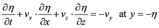 (03)
(03)
and as dynamic condition
 (04)
(04)
applies to the fixed boundary (bottom)
 . (05)
The basic differential equation system for the flows under consideration is thus from Equations (01) to (05).
![]()
Figure 1. Flow with bottom and free surface.
4. Perturbation Theory
4.1. Development of the Perturbation Parameter and Introduction Dimensionless Variables
For the futher developments a formal perturbation procedure is used, which is developed in this form of Friedrichs [2] and also described in [3] . Friedrichs with this perturbation method successfully derived the equation of shallow water theory (Saint-Venant equations without friction) from the Euler equations for incompressible flows as an approximation in the lowest order to the solution of the potential theory. Together with Hyers Friedrichs [4] succeeded also to develop from the potential theory the equation of the solitary wave as a second approximation, taking into account the higher terms of the perturbation theory. Similar developments can also be found in [5] .
For the application of the disturbance producer, the definition of a perturbation parameter is of crucial importance. For the present partial differential equation system, it is advisable to use the kinematic viscosity of fluid  [m2/s] as the decisive fluid property, the acceleration due to gravity g [m/s2] and an arbitrary depth
  [m]. With these physical quantities the dimensionless parameter can be formed
 (6)
(6)
which can be considered as a dimensionless kinematic viscosity in an earthly gravity field. Taking into account the developments in [1] , the following dimensionless variables are now introduced which are initially marked with (*):
![]() (7)
(7)
![]() (8)
(8)
![]() (09)
(09)
![]() (10)
(10)
To form the dimensionless pressure, the density ![]() [kg/m³] of the liquid is additionally used.
[kg/m³] of the liquid is additionally used.
For the transformation of the variables, the following relationships are used:
![]() (11)
(11)
![]() (12)
(12)
![]() (13)
(13)
![]() (14)
(14)
![]() (15)
(15)
![]() (16)
(16)
![]() (17)
(17)
![]() (18)
(18)
![]() (19)
(19)
![]() (20)
(20)
![]() (21)
(21)
![]() (22)
(22)
![]() (23)
(23)
![]() (24)
(24)
![]() (25)
(25)
![]() (26)
(26)
![]() (27)
(27)
![]() (28)
(28)
![]() (29)
(29)
![]() (30)
(30)
![]() (31)
(31)
![]() (32)
(32)
![]() (33)
(33)
![]() (34)
(34)
![]() (35)
(35)
![]() (36)
(36)
In the next step, the newly defined variables are inserted in the system of differential Equations (01) to (05). In addition, is dispensed with the identification of new variables by (*).
From the continuity Equation (01) results in
![]() (37)
(37)
respectively
![]() . (38)
. (38)
From the momentum Equations (02a) to (02c), we obtain
![]() (39)
(39)
respectively
![]() (40)
(40)
![]() (41)
(41)
respectively
![]() (42)
(42)
![]() (43)
(43)
respectively
![]() . (44)
. (44)
Equations for the boundary conditions maintain the form
![]() (45)
(45)
respectively
![]() (46)
(46)
![]() (47)
(47)
and
![]() (48)
(48)
respectively
![]() . (49)
. (49)
As a result, the basic system of differential equation takes the form
![]() (01)'
(01)'
![]() (02a)'
(02a)'
![]() (02b)'
(02b)'
![]() (02c)'
(02c)'
![]() (03)'
(03)'
![]() (04)'
(04)'
![]() . (05)'
. (05)'
4.2. Analysis of the Developed System of Differential Equations
The selected perturbation parameter represent, for example, for liquid water with ![]() at a temperature of 10˚C a very small quantity, even for a depth in the mm range
at a temperature of 10˚C a very small quantity, even for a depth in the mm range![]() . It follows that by perturbation parameter
. It follows that by perturbation parameter ![]() and by powers of
and by powers of ![]() the individual terms of the equation system are assigned different order of magnitude, and thus these terms have different signification. This is particularly evident in the outstanding effect of the pressure and the pressure gradients. Also it can be seen that all gradients in the vertical
the individual terms of the equation system are assigned different order of magnitude, and thus these terms have different signification. This is particularly evident in the outstanding effect of the pressure and the pressure gradients. Also it can be seen that all gradients in the vertical ![]() - direction have a smaller effect than the gradients in the horizontal direction and that the local accelerations terms have a smaller magnitude than the convective acceleration terms.
- direction have a smaller effect than the gradients in the horizontal direction and that the local accelerations terms have a smaller magnitude than the convective acceleration terms.
The next step is to assume power series developments for ![]() and
and![]() :
:
![]() (50)
(50)
![]() (51)
(51)
![]() (52)
(52)
![]() (53)
(53)
![]() (54)
(54)
and insert them in the Equations (01)' to (05)'. The aim is to obtain, by equating coefficients of like powers of![]() , equations for the successive coefficients in the series
, equations for the successive coefficients in the series
For example, the terms of zero order ![]() yield the equations
yield the equations
![]() , (01)'0
, (01)'0
![]() , (02a)'0
, (02a)'0
![]() , (02b)'0
, (02b)'0
![]() , (02c)'0
, (02c)'0
![]() , (03)'0
, (03)'0
![]() , (04)'0
, (04)'0
![]() . (05)'0
. (05)'0
It turns out that only with mathematical results of the approximation of lowest order, such as with the result that the pressure in ![]() -direction is equal to zero, no results could be found which are consistent with the physical reality.
-direction is equal to zero, no results could be found which are consistent with the physical reality.
In the next step we are considering the first order![]() . This terms arising from (01)' to (05)' in their turn yield the equations
. This terms arising from (01)' to (05)' in their turn yield the equations
![]() , (01)'1
, (01)'1
![]() , (02a)'1
, (02a)'1
![]() , (02b)'1
, (02b)'1
![]() , (02c)'1
, (02c)'1
![]() , (03)'1
, (03)'1
![]() , (04)'1
, (04)'1
![]() . (05)'1
. (05)'1
From these equations of the first approximation Equation (02b)'1 can easily be integrated at once. With the boundary condition that the pressure is zero at![]() , the following
, the following
![]() (55)
(55)
which is obviously the hydrostatic pressure relation in dimensionless form.
The terms of second order ![]() yield the equations
yield the equations
![]() , (01)'2
, (01)'2
![]() , (02a)'2
, (02a)'2
![]() , (02b)'2
, (02b)'2
![]() , (02c)'2
, (02c)'2
![]() , (03)'2
, (03)'2
![]() , (04)'2
, (04)'2
![]() . (05)'2
. (05)'2
It can be seen that in the second approach no linear pressure distribution is available.
Finally, it is clear that the method presented new systems of equations arise which offer new possibilities of solutions for physical problems that are related to the Navier-Stokes equations.
5. Example: Stationary Open Channel Flow
The application of the developed approximation systems shows the following, the derivation of an equation for the stationary open channel flow (Figure 2).
For this flow the Equation (02b)'1 gives
![]() . (56)
. (56)
Similarly, it follows from the equations
![]() . (57)
. (57)
![]()
Figure 2. Stationary open channel flow [6] .
If ![]() is introduced by constant slope
is introduced by constant slope ![]() of the channel, is obtained furthermore from the Equations
of the channel, is obtained furthermore from the Equations
(56) and (57)
![]() . (58)
. (58)
From Equation (02a)'1 result
![]() , (59)
, (59)
since from Equation (01)'0 follow ![]() and thus
and thus
![]() . (60)
. (60)
Combining Equations (58) and (59), we obtain
![]() . (61)
. (61)
In the following, the channel flow will now be considered in the coordinate system ![]() (Figure 2) [3] . The relationship between
(Figure 2) [3] . The relationship between ![]() and
and ![]() follows from
follows from
![]() (62)
(62)
and with ![]() is obtained at the usual slope of channel
is obtained at the usual slope of channel
![]() (63)
(63)
Considering these relationships the integration of Equation (61) yields
![]() . (64)
. (64)
As a boundary condition at the free surface of water at ![]() is obtained for the shear stress between water
is obtained for the shear stress between water
and air ![]() and thus is also
and thus is also ![]() at this point equal zero. It follows
at this point equal zero. It follows
![]() (65)
(65)
respectively
![]() . (66)
. (66)
The integration yields
![]() (67)
(67)
and with the no-slip condition, according to ![]() and
and![]() , is also
, is also![]() .
.
Finally, the back transformation of Equation (67) to variables with dimension yields
![]() (68)
(68)
![]() (69)
(69)
It is apparent that equation for laminar channel flow can be viewed as an approximation of the lowest order of the Navier-Stokes equations for incompressible flows.
6. Conclusion
Partial differential equation systems consisting of the Navier-Stokes equations, the equation of continuity and equations of the relevant boundary conditions can be represented by the perturbation theory in dependence of a dimensionless parameter, which is introduced as a reciprocal of the Reynolds number. From the relations arising from the comparison of the coefficients of this parameter, approximate solutions of different orders can be developed for the initial system.