Power Balance of Multi-Harmonic Components in Nonlinear Network ()
1. Introduction
Two types of mixing circuits containing three main harmonic components are introduced in this paper. The first type uses two signal sources with frequencies (w1, w2) which are not the integer multiple of each other for mixing. The positive conductance with quadratic characteristic is used as a frequency conversion device to generate difference frequency (w2-w1). There is only power-wasting positive resistance in the circuit, and self-excited oscillation cannot be produced. Three main harmonics are solved by frequency domain balance theorem and circuit law, and the complex power of each frequency component is individually conserved. The correctness of solving results is confirmed by traditional harmonic analysis method. The frequency components besides two signals will be produced in nonlinear circuit, for example there is no difference frequency excited source in circuit, but the power consumption of difference frequency component in the network can still be balanced. The power calculation in mixing circuit has important theoretical significance. It indicates that the balance theorem of frequency domain is applicable to not only odd term equation, but also even term equation. Circuit parameter design makes difference frequency component occupies a sufficient proportion in the overall mixing output, which has an important practical value.
The second type uses a nonlinear element with negative conductance and cubic characteristic. The circuit includes three main frequency components, the self-excited oscillation and two signal frequencies. The timedomain solution is expressed as the frequency-domain solution of Fourier series. There is no mathematical abstraction transformation formula for selecting appropriate harmonic term, so it can only rely on the physics background for establishing equation. The correct harmonic component can be sought by complex power balance theorem. This paper propels the application of theorem from single first harmonic to containing three main harmonics [1] -[8] . The mixing circuit structures of two types are identical, and only the various device parameters in the circuit and nonlinear characteristics are different. The interaction relation of nonlinear couplings of three main harmonics, and the calculation formulae of the first and second types are completely different.
2. First Type Mixing Oscillation—Difference Frequency Is Main Harmonic Component
2.1. Three Main Harmonics Solved by Harmonic Analysis
Symbols used in this paper are as follows, taking variable  as example,
  or the subscript v represents phasor,
 . The subscript
  denotes amplitude, the
  denotes real part, the
  denotes imaginary part. For nonlinear branch,
  denotes instantaneous current,
  denotes the harmonic
  component of the
 , while
  denotes the phasor of
 , the
, the  denotes amplitude,
  denotes active component,
  denotes reactive component,
  denotes the phasor of
 , the
, the  denotes the current phasor of difference frequency
 . The electrical engineering symbol j is used as the imaginary unit in this paper, for example, the phasor
  in Example 1, and the phasor
  in Example 2.
Example 1: The state equation of mixing model in Figure 1 is shown in (1), the scalar equation is shown in (2).
 ,
,  ,
,  ,
, (1)
(1)
 (2a)
(2a)
 (2b)
(2b)
 (2c)
(2c)
 (3)
(3)
The variable u contains a large number of frequency-doubling and combined-frequency components besides the two signal frequencies. In order to strengthen this available difference frequency component, the resonant frequency of LC circuit is designed to be equal to the difference frequency  as shown in (2b). The excited source
  is shown in (2c). The three main harmonic components
  are set as shown in (3), where
  and
and  denote two signal frequencies, and
  denote difference frequency. The
 ,
,  ,
,  ,
,  ,
,  ,
,  are six undetermined coefficients. The LC circuit cannot produce self-oscillation while is used as selective filter circuit. Its task is to select difference frequency from the numerous frequency components of mixing. If the two excited sources are removed, namely let
  then w12 cannot maintain self-excited. The difference frequency component relying on the two excitation support is not self-oscillation. It is commonly known as mid-frequency. The data of three main components are found by Program Tab1.nb, as listed in Table 1, where % represents the percentage of difference frequency in all outputs, maxu represents the maximum total output.
2.2. Result Verified by Power Balance Theorem
The node method is used, and only one node voltage u contains three harmonic components in circuit Figure 1. The u is the variable of differential Equation (1), and the node voltage-phasor equation of three main harmonics is listed, as shown in (4).
 ,
, (4a)
(4a)
 (4b)
(4b)
 (5a)
(5a)
 (5b)
(5b)
 (5c)
(5c)
 ,
,  ,
, (6)
(6)
The (4) represents the current balance equations of three components according to node method denoted by phasor. If it is linear conductance , then
 , and every harmonic component of node voltage u can be independently solved by (4). There is no difference frequency component:
  and
and  at this time. However,
  is the non-linear conductance, and
  is related to not only
  but also
 ,
, . The coupling relation among three harmonic components is obtained by Program coupling.nb, as shown in (5). The current of a harmonic component includes the contributions of other harmonic voltage components. Therefore, the solution should be jointly found by (4) and (5). The real and imaginary parts of every phasor equation should be equal individually, so six equilibrium equations can be set up, six undetermined coefficients can be jointly solved as well. The data obtained by Program Power1.nb and Tab1.nb are consistent, as shown in Table1

Table 1. Main harmonic solution of Example 1.
Finally, every harmonic power sum given by the program is identically equal to zero. It is verified that the power profit and loss of each harmonic component cannot be mutually replenished and will be individually conserved. The (5) can be represented as the general form shown in (6).
It should be pointed out that there is no difference frequency excited source in the circuit Figure 1. The power consumed by the difference frequency component in the positive conductance  is supplied by the nonlinear element
  of variable-frequency. Taking the Table 1(e) as example, the
  which represents the active power consumed by branch
  is negative as shown in (7). The
  which represents the active power consumed by branch
  is positive, as shown in (8). The active power consumed by
  and
and  is completely balanced. The currents of branches L and C from difference frequency component are equal in size and opposite in direction. The consumed reactive power totals zero, as shown in (9).
 ,
,  ,
, (7)
(7)
 ,
,  ,
, (8)
(8)
 (9)
(9)
The operation results of the Program Power1.nb show that the nonlinear element  only consume active power, three main harmonics do not consume reactive power
 .
.
2.3. Frequency Conversion and Power Conservation
After frequency conversion, the conservation theorem still is valid. Taking the transformer as an example shows the principle of variable-frequency. For example, high-voltage (6.3 kV) generator sends power to low-voltage (380/220 volts) users through a step-down transformer. Moreover, the power sent by generator and the power received by transformer on high-voltage side (including internal transformer consumption and power transformed into low voltage side) should be balanced. The power sent by low voltage side should be equal to that consumed by user. The power sum of two voltage levels should be individually balanced in this electric network. Transformer is a power source of the user on the low voltage side, but transformer itself does not produce power. It only plays the role of transforming high-voltage power into low-voltage power.
Industrial users of containing frequency conversion device use other frequencies to consume power. However, the power company sends 50 Hz frequency power to users, and then frequency conversion device will receive 50 Hz power. Therefore, the power system should maintain the complex power balance of 50 Hz frequency component. The power of frequency component after conversion should also maintain its power balance.
Two excited sources send power to the network containing frequency conversion element. Moreover, power sent by two excited sources using excited frequency and the power received by network (including the power consumption of internal network and the power transformed into difference frequency) should be balanced. The difference frequency power sent by frequency conversion element should also be equal to the power consumed by positive resistance. The power sum of three frequency components should individually be balanced in this electric network.
3. Second Type Mixing Oscillation
3.1. Three Main Harmonic Solved by Harmonic Analysis
 ,
,  ,
,  ,
,  ,
,  ,
,  ,
,  ,
,  (10)
(10)
 ,
,  ,
,  ,
,  ,
,  ,
, (11)
(11)
 (12a)
(12a)
 ,
, (12b)
(12b)
 ,
,  ,
,  ,
, (13)
(13)
 (14a)
(14a)
 ,
,  ,
, (14b)
(14b)
Example 2: Circuit is shown in Figure 1. Each element parameter are shown in (10), they is different from Example 1. The state equation is shown in (11), scalar equation is shown in (12). The comparison between state (11) and (1) shows that the two equations are identical in form, the comparison between scalar (12a) and (2a) shows that the two equations are also identical in form, and only their parameters and nonlinearities in the formulae are different, where ,
,  ,
, .
.
Let , the self-oscillation
  still exists due to
  has negative conductance term. The
  of the harmonic
  of self-oscillation are solved by Program Self.nb, as shown in (13), where
  denotes amplitude of self-oscillation when
 . The initial phase angle
  is arbitrary, it means the harmonic solution has no determined
 . The self-oscillation of nonlinear circuit tends to a stationary limit cycle after the transient process. The circuit entering steady state certainly possess a transient time
  later from beginning. The initial phase angle
  of first movement of entering steady state cannot be determined. The
  and
and  depend on different initial conditions, they cannot be sought. The stationary oscillation solution can be sought by harmonic analysis and power equilibrium theorem. The transient process is not an oscillation solution before entering limit cycle, which does not consist of harmonics and thus cannot be found by the harmonic analysis.
Let , three main harmonics containing self-oscillation are obtained by Program uhp.nb, as shown in (14). The comparison between (14) and (3) shows that the two formulae are also identical in form, and only their coefficients in the formulae are different, where
 .
.
The solutions of self-excited and forced oscillation can be sought by superposition in linear equation. The coupling solution of self-excited and forced components should be jointly sought by Program uhp.nb.
Note that the self-excited oscillation is inhibited and disappears due to nonlinear coupling interaction when the combination strength of the  is strong enough [9] -[12] . At this time, setting the
  in (14), and two main harmonics containing only forced oscillation are obtained by Program onlyup.nb.
The results solved by Programs uhp.nb and onlyup.nb are listed in Table2
Table 2. Main harmonic solution of Example 2, .
.
It should be noted that the initial value is not introduced, but the self-oscillation amplitude  solved by Program uhp.nb has determined. However, the
 , the
, the  cannot be specifically determined. Therefore, the
  is multi-solution. Above is shown in Programs uhp.nb and Table2
 ,
,  ,
,  (15)
(15)
 ,
,  ,
, (16)
(16)
 ,
,  ,
, (17)
(17)
The mutual coupling relationship among three main harmonic components is shown in (15)-(17). One of harmonic current includes the contributions of the other harmonic voltage components. The concepts and definitions of equivalent voltage amplitude  can be formed by (15), the equivalent conductance
  can be defined by (16), and The current
  of self-oscillation in (17) is equal to the product of self-oscillation voltage and equivalent conductance
 , where
  contains the contributions of other harmonic voltage.
The initial condition is not introduced by the two examples in this paper, thus merely steady state solutions can be found. However, the distinction between difference frequency and self-oscillation components can be shown by the (5) and (17). In the (5),  and
and  are from the conversion of the excited source, they disappear when
 , therefore the
  is forced component, is unique determination. But in (17), the
  and
and  are self-oscillation component, their power are not from the excited source, they still exist when
 , thus the
  is unique determination, while the
  is multi-solution.
3.2. Using Phasor Method and Power Balance Theorem
Using phasor method and frequency domain balance theorem (including frequency domain KCL and KVL as well as power equilibrium theorem) can obtain the conclusions which are consistent with those of harmonic analysis.
Firstly, let , the
, the  can be obtained by fundamental wave equilibrium principle, as shown in (13). If self-oscillation component exists, then mutual relationship among
  and four unknown coefficients
  is shown in (15) and (18).
 ,
, (18)
(18)
 ,
,  ,
, (19a)
(19a)
 ,
,  ,
, (19b)
(19b)
Secondly, if , the current equilibrium equation of two forced components is set up by using node method denoted by phasor, as shown in (19). The
  and
and  in the above formulae are related to the voltage amplitudes of three harmonics, as shown in (16). The real and imaginary parts must individually be equal for each phasor equation, so four equilibrium equations can be set up to solve jointly four undetermined coefficients. The solutions from Programs haveself.nb are consistent with Program uhp.nb.
The equivalent conductance  for
for  is only relevant with the equivalent voltage amplitude
  as shown in(16), the
 only depends on the specific parameters of network; and is irrelevant to the excited
 . The
. The  independent from initial phase angle
 , while the
  depends on the initial conditions, Therefore the
  independent from initial conditions.
If , and the self-oscillation does not exist when the
  is strong enough. The solutions of the (12) only contain two forced component, they can be obtained by Program nonself.nb. They are consistent with the solutions by Program onlyup.nb. All results obtained by phasor method and by harmonic balance method all are consistent, as shown in Table2
3.3. Existence of Self-Oscillation Depending on Power Balance Conditions
 ,
,  ,
,  (20)
(20)
If , the (20) can be obtained from (18), then
  when self-oscillation exists. If
  is obtained, it indicates that the self-oscillation has disappeared for stronger uF. Whether self-oscillation exists can be determined by using the (20). Self-oscillation exists when
 ; self-oscillation disappears when
 .
.
3.4. Incongruous with Power Balance Conditions Results in Wrong Conclusion
The first case suppose harmonic solutions contain self-oscillation component, the wrong result will be obtained when external excited source is larger such as ,
, . We obtain the imaginary
 . The
. The  is found by Program uhpwrong.nb, so it can be determined by (20) that the self-oscillation has disappeared. The harmonic solutions should be reset, and self-oscillation component is removed. The correct results in Table 2(e) can be obtained by Program onlyup/E.nb.
The second case suppose harmonic solution exclude self-oscillation component, the wrong result will also be obtained when external excited source is small such as ,
, . It can be determined that selfoscillation exists according to (20). we can obtain the (21) from Program upwrong.nb.
 ,
, (21)
(21)
The harmonic solution should be reset as including self-oscillation, and the correct results in Table 2(b) can be obtained by Program uhp/B.nb. The solution set by harmonic analysis is a trial solution. It has very important significance that the containing harmonics component are estimated from the physical background.
In the first case, the results satisfying the equation equilibrium are all complex roots when  is larger and errors obviously exist in them. For the second case, set harmonic component only contains two main harmonics, and real solution can also be obtained, as shown in (21). In order to find such hidden error, it is necessary to understand the physical background containing self-excited oscillation. Whether this solution is correct should be verified according to the (20) and (21).
4. Two Types of Oscillation Characters
4.1. Phase Portrait of First Type Mixing Oscillation
There is no negative conductance to release energy, so there is no self-oscillation component. Two excitation signals are finite energy source, and their mixing oscillation outputs are bounded. Periodic oscillation or chaos may be formed. The  plane phase portraits of overall output of mixing oscillation are drawn by Simulink. Taking Table 1(e) as an example, phase portraits are shown in Figure 2, where Figure 2(a) takes 100% of the phase points, and Figure 2(b) takes the last 5% of the phase points. They cannot show intuitively periodic or chaotic state.
In order to judge phase portrait property, the (1) and (2) are converted into three-dimensional state equation as shown in (22a), the phase portrait behavior is verified by Lyapunov Exponent (LE). Jacobi matrix is shown in (22b), where  denoted by (2c).
 ,
,  ,
,  ,
, (22a)
(22a)
 (22b)
(22b)
 ,
, (23)
(23)
 ,
,  ,
,  when
when  (24)
(24)
 ,
,  ,
,  when
when  (25)
(25)
The operation of LE program takes initial value at  as shown in (23). It can be found that the maximum Lyapunov Exponent LE3 is positive when the operation time
  is shorter as shown in (24). The phase portraits show a chaotic state as shown in Figure 2(a). While LE3 tends to zero when the operation time
  is longer, as shown in (25). The LE have two negative and one zero when running time is long enough, and a periodic state appears as shown in Figure 2(b). The phase portrait evolves and converges to the
 (a)
(a) (b)
(b)
Figure 2. The  plane phase portrait of Table 1(e). (a) Drawing for 100% phase points; (b) Drawing for last 5% phase points.
final periodic state from chaotic state at the beginning.
There is only forced oscillation in this circuit entering steady state, and there is no freedom self-oscillation. Finally, freedom component inevitably exhausts to zero because there is only positive resistance element in the network. Excited source energy export to the third harmonic (difference frequency) through frequency conversion. These three harmonic components occupy predominant positions in the Fourier series expansion. The results from combined excitation of two signal sources are equivalent to a non-sinusoidal periodic source including two harmonic components  and
and . If calculation is strict and accurate, then common base frequency is
 , and period is
  seconds (if MATLAB operation can achieve such precision). Various harmonic components are the integer multiples of
 . When the simulation time
  or LE operation time
 , phase portrait plotted hasn’t finished one cycle, it is shown as aperiodic chaos.
If such high precision is not reached when the phase portrait is drawn by Matlab numerical simulation, the drawn phase portrait may become periodic state when w1, w2 mantissa 0.01 is ignored, and cycle is T = 6.2832 second. Therefore, the precision of numerical simulation will also affect the character of phase portrait.
The oscillation behaviors for the overall output of mixing circuits can be divided into two kind of pattern of the periodic and chaotic state. However, the data handled by Matlab are all rational numbers, so the drawn phase portrait is all periodic track. In fact, there is only periodic function when the phase portrait is drawn by numerical simulation. The chaotic oscillation can be considered as sufficient or infinite extension of period T.
4.2. Phase Portrait of Second Type Mixing Oscillation
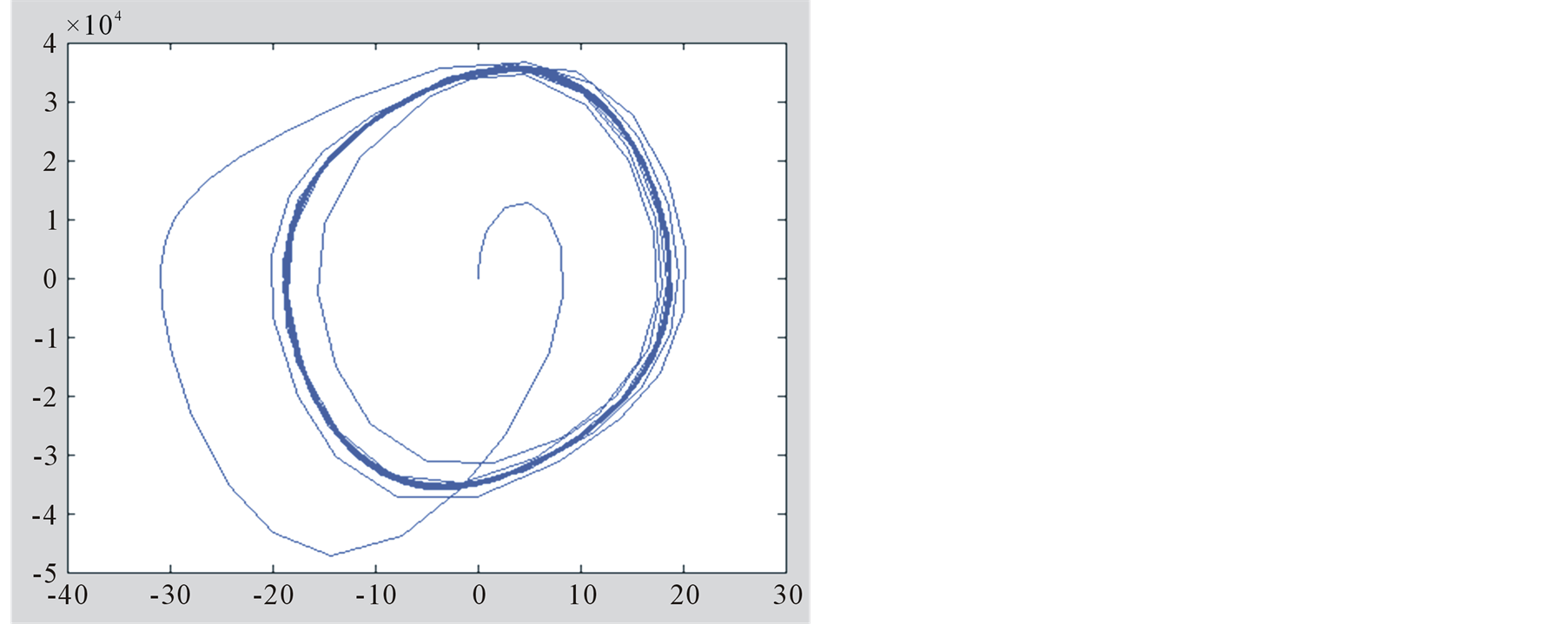
Taking the Table 2(a) as an example, the  plane phase portrait of overall output of mixing oscillation is drawn by Simulink, as shown in Figure 3. The Figure 3(a) takes 100% phase points, and Figure 3(b) takes the last 1/1000 phase points.
It is clear that distinguishing chaotic or periodic state cannot be directly perceived. The phase portraits of the mixing oscillation are either chaotic or periodic states. If their cycle lengths are moderate, neither very short nor very long, distinguishing strictly the oscillation behavior is difficult. The phase portrait characters are closely related to the simulation time. The phase portrait appears non-periodic when simulation time TS is shorter than one complete cycle T. The phase portrait shows periodic state when the simulation time TS is bigger than T. It can be seen from this example that the mixing circuits containing self-oscillation usually produce chaos, namely the TS smaller than T.
4.3. Phase Portrait of Single Excitation
Taking the Table 2(g) as an example, the  plane phase portrait of oscillation caused by single excitation is drawn by Simulink, as shown in Figure 4. The Figure 4(a) takes 100% phase points, it contains transient process of the oscillation; and Figure 4(b) takes the last 1/1000 phase points, it only contains the process after entering steady state.
Non-linear oscillation refers to vibration with sustained oscillation character. It can be divided into two categories. One is periodic oscillation or constant periodic oscillation, in which dynamic variable tends to be steady with periodic repeatability. This kind of oscillation can be expressed as Fourier series. Another one is called non-constant periodic oscillation or aperiodic oscillation for short. Dynamic variable in such oscillation will keep oscillating continuously but without determination period. Although the orbit in phase portrait is without repetition, however the oscillation is sustained. Such a phenomenon is called aperiodic oscillation.
The example in Table 2(g), the oscillation can be divided into transient and steady state processes. The transient process belongs to aperiodic oscillation; the steady state process belong to periodic oscillation. For some nonlinear system, the aperiodic process can be extended infinitely or sufficiently. Within whole simulation time, aperiodic oscillation is unique state instead of temporary part of whole process, this is chaos. It is a very common bounded nonlinear function. The whole process of the oscillation cannot be divided into transient and stead-state.
It is another leap that human understands nature. The parasitic oscillation phenomenon, such as a mess on display had been found in nature a long time ago. It is difficult to distinguish that the mess are periodic or chaotic oscillations.
 (a)
(a)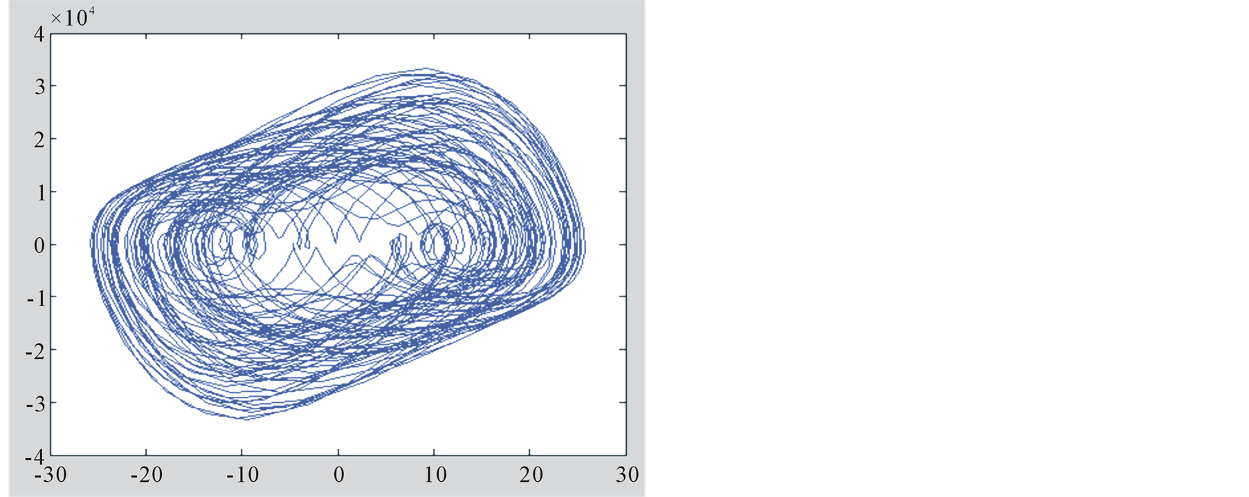 (b)
(b)
Figure 3. Phase portrait of Table 2(a). (a) Drawing for 100% phase points; (b) Drawing for last 1/1000 phase points.
 (a)
(a)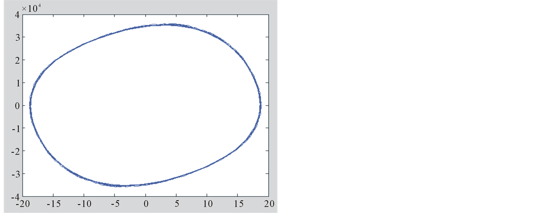 (b)
(b)
Figure 4. Phase portrait of Table 2(g). (a) Drawing for 100% phase points; (b) Drawing for last 1/1000 phase points.
5. Conclusions
1) In domestic and foreign literature, with regard to researching nonlinear circuits and chaos all are established on the basis of dynamic mechanics except the mathematic method of finding differential equations. The complex power balance theory opens up a new field for researching nonlinear oscillation. The correct harmonic components can be sought by power balance theorem of frequency domain. This paper propels the application of theorem to containing three main harmonics from single fundamental wave in the past.
The operation results of two kinds of programs (Tab1.nb and Power1.nb; uhp.nb and haveself.nb; onlyup.nb and nonself.nb) are consistent. It shows the pervasiveness of application of complex power balance theorem.
2) The chaos can be researched from the theory of frequency domain. This is an importance contribution of power balance theory. This paper propels the application of theory to chaotic oscillation. The main part of the steady-state oscillation solution is obtained through the power balance theory, its important contribution shows that the main harmonic solution is able to represent the basic part of both periodic solution and chaotic solution. Even though chaos is non-periodic within simulation time, its basic main part is periodic, and the main harmonic balance equations belong to linear equations.
3) The necessary and sufficient condition for periodic oscillation is that there should and must be only one unique common fundamental frequency. If there is no unique single common fundamental frequency, such as Chua’s circuit, Lorenz system, Chen system, Lu system, Liu system, Qi system, etc., because their solutions cannot be expressed in Fourier series, they all belong to aperiodic chaotic oscillation.
If there are more than two main harmonic waves in the circuit, chaotic oscillation is possibly produced. The phase portraits in Table 2(a)-(c) show that chaos usually can be produced by the mixing of multi-harmonic. The more the harmonic components of involving mixing are, the greater the possibility of producing chaos is.
4) Steady-state oscillation solution is obtained through the harmonic-coefficient balance formulae of differential equation. Its roots may contain more than ten groups sometimes. A reasonable solution should be selected by power balance theorem. The complex power of every harmonic component totals zero. There is no self-excited oscillation if the amplitude meeting power balance requirements is an imaginary root . The (20) can be used to determine whether there is self-excited oscillation, and thus a very reliable result can be got. Its correctness can be verified with the phase portrait.
5) There are two types of harmonic components of non-excitation frequency in the network. One is the selfoscillation frequency. Its power is produced by the non-linear element  with the characteristic of comprising negative term as shown in (11), and it can produce power by itself without excitation source. The greater the voltage amplitude is, the smaller the power produced by the
  of comprising negative term is. The power produced by the
  is insufficient to compensate the consumed power in positive conductance
  when amplitude increases up to a certain value, then self-excited oscillation disappears.
The other harmonic component is produced by variable frequency element of containing only positive characteristics as shown in (1), and it cannot produce power by itself without excitation source. It only plays transformation action. The power consumption of difference frequency component cannot be directly replenished from the power exported by excited source. It is necessary to convert excited power into the power of difference frequency component through frequency conversion element. The variable-frequency element is the source of difference-frequency power which is produced by its transformation instead of directly by itself. The difference frequency component of non-excited frequency always exists, when amplitude increases up to sufficiently large.
Acknowledgements
This work was supported by National Natural Science Foundation of China (60662001).