Role of Accessibility and Socio-Economic Variables in Modelling Population Change at Varying Scale ()
1. Introduction
The agglomeration of society can be generally explained by the economies of scale, positive feedback in circular causation, and increasing returns [1] . However, the importance of accessibility to the economic development and urbanisation at a regional level is evident [2] [3] . The role of accessibility and its effects on the development of various types of areas have been considered in a great number of studies using different types of indicators, and extensive reviews have been produced on the subject [4] -[6] .
Even though there is no full agreement on the effects of accessibility, some general principles or key findings may be identified. For example, according to Krugman [7] , the emergence of a core-periphery pattern depends on transportation costs, economies of scale, and the share of manufacturing in national income. According to Vickerman et al. [8] , the relative gains in accessibility of peripheral regions may be beneficial to their economic development, but these gains will always be over-shadowed by the much larger gains in accessibility of the regions in the core. Fujita and Thisse [9] state even more specifically, that there is a fundamental trade-off between scale economies and transportation costs in the geographical organisation of markets, and low transport costs tend to favour the formation of geographical clusters or to deter the creation of new ones. In addition, densely populated industrialised areas tend to have a higher network infrastructure endowment in comparison to peripheries [10] . However, the effect of road investments do not necessarily affect accessibility to a remarkable extent due to increasing travel volumes, and also the welfare gains may prove to be fairly modest in terms of travel time and costs [11] .
Several empirical studies underpin the agglomeration trend in society, as accessibility is related to population dynamics in the centre-periphery pattern [12] -[14] . Also, the location choices of companies are seen to be affected by accessibility [15] . While the importance of accessibility to regional development is evident the actual causality of the relationship is, however, more complicated, since the effects of accessibility are not completely straightforward [16] . For the economic development of a region, good infrastructure is evidently a precondition, and equally good infrastructure at neighbouring regions seems to promote the growth too. However, investments to already good infrastructure do not stimulate the growth and positive effects of investments wane quickly in time. Moreover, the support of political, policy and institutional factors is essential to the growth process [17] and consumption amenities may greatly affect the success of centres competing for population [18] .
Even though the role of accessibility in general is rather clear in the developments related to the centre-periphery pattern, the regional pattern may be stirred by the trends related to counter urbanisation, in which [19] identifies differing trends of anti-urbanisation, displaced urbanisation and ex-urbanisation. In terms of accessibility, the question pertains to the two latter phenomena, as population growth on the urban fringe is related to improved accessibility [20] , and particularly to increasing motorisation, under conditions of increasing incomes and employment [21] .
As the geographic space is usually ignored in demographic research, there is a need to bring spatial processes explicitly into empirical demographic studies to correct any potential misspecifications [22] . Traditionally, population change is analysed with birth and death rates connected to net migration and possible correction factors. The research in this field has produced an amply set of highly sophisticated statistical models [23] [24] . In contrast, land-use dynamics, such as urban growth, are modelled by spatial variables also including distance-based indicators [25] [26] .
Watson [27] has observed that geographers tend to work at one analytical level exclusively and implicitly, without considering other alternatives. However, changes in scale change the importance and relevance of variables [28] . High-level aggregation at coarse scales can obscure the variability of units and processes and is inaccurate for fine-scale and local assessments [29] . Also, problems related to ecological fallacy may be encountered. The choices over scale, extent, and resolution in the analysis may critically affect the type of patterns that will be observed [30] . Hence, it is important to take Marceau’s [31] claim into consideration, that it is necessary to identify scale thresholds to understand the interactions occurring within and between the levels of organisation.
2. Research Design
In this paper, the performance of accessibility and socio-economic variables in explaining population change are studied by multi-scalar approach in the case of Finland. Specifically, the study seeks to define the relevance of accessibility and socio-economic variables in explaining population change in relation to scale. The research questions are stated as follows: 1) What are the essential accessibility and socio-economic variables in explaining population change at different scales? 2) What are the characteristics of the relationship between these variables and population change in relation to scale? 3) How well can population change be modelled statistically at different scales using accessibility and socio-economic variables? 4) How does the scale affect the explanatory importance of each variable?
Methodologically this paper relies on the use of geographic information systems (GIS) in spatial data management, variable construction, and statistical techniques in establishing models for predictive or descriptive purposes. The modelling will be based on an empirical-statistical approach and perceived empirical relationships, which will be subsequently used in constructing the predictions. In contrast to analytical-theoretical and mechanistic-process models, this approach does not attempt to mathematically formulate theoretical models or to describe actual causalities [32] .
As yet, only a few studies have considered the effect of accessibility on population dynamics in Finland. The setting of this study emanates from a finding by Kotavaara et al. [33] [34] , indicating that there appears to be a strong and continuous relationship between accessibility potentials and population change in Finland since the 1990s. Indeed, potential accessibility based on travel by car seems to be an important variable in explaining this trend of population concentration at a local scale, but due to the lack of socio-economic data, the omitted variable problem is potentially present in previous studies [35] .
The study makes use of digital transport infrastructure models and register-based 1 km × 1 km population and socio-economic grid cell data from Statistics Finland, which is available independent of administrative boundaries. Accessibility computations, spatial analyses and data management are carried out using GIS. In analysing relationships between population change and explanatory variables, a non-linear multiple regression technique, generalised additive models (GAMs), was applied. In establishing models, a large set of variables were constructed and tested by extensive preliminary analysis which included accessibility potentials based on six distance decay functions, accessibility of air and rail transport facilities and 58 socio-economic variables. Two accessibility and four socio-economic and population density variables were selected for the final statistical models on the basis of theoretical consistency and explanatory power in the univariate and multivariate context.
As the scale is an important factor for the modelling performance, and any grid cell resolution has not proved to be particularly applicable for modelling population change, six different resolutions (2, 4, 8, 12, 16 and 24 km) were used. The smallest grid size, 2 km × 2 km, was the most accurate resolution at which the calculation of accessibility potentials was computationally possible, whereas the 24 km × 24 km resolution is roughly equivalent to the municipal division in terms of spatial resolution. The population change was analysed between the years 2003 and 2009, determined by the availability of data. In addition to analysing relationships and importance of accessibility and socio-economic variables, the predictive ability of the models was evaluated at all resolutions.
3. Finnish Context of Research
Finland is a very suitable study area for analysing the effect of accessibility on population change, together with some key socio-economic variables. A substantial benefit to the analyses of this study is gained from the availability of accurate population and transport network data enabling an accurate scale analysis. Scrutinising population dynamics on a grid cell basis has a long tradition in Finland [36] . However, despite dedicated research efforts aimed at understanding population dynamics, demographic trend calculations are the only actual spatial models representing the population change in Finland. The case of Finland is an opportunity for the understanding of urbanisation in sparsely populated and peripheral countries, which differs from the typical setting of urbanisation in Western Europe and Northern America.
Finland urbanised late in comparison to the rest of Europe. Urbanisation and motorisation occurred during the 1960 in Finland whereas in many other countries the same period is characterised by suburbanisation instead. Finland has also experienced a remarkable structural change in the economy over the past few decades. The economy has opened up to global markets since the collapse of the trade with the Soviet Union and the membership in the European Union in the mid 1990s. Simultaneously, the focus of regional development policies was gradually shifted from supporting and subsidising peripheries and degenerating regions to developing centres [37] .
Finland is characterised by long internal distances and traffic has been dominated by the use of private cars. Public transport is available mainly within and between urban areas, effectively leaving large areas without service. Because of the remote northern location and the border with the Baltic Sea, Finland has had limited connections with other countries, in comparison to many other European countries [38] .
The Finnish road network was essentially built to its present coverage during the 1960s and the 1970s. There has been only a slight increase in the average vehicle speeds on the Finnish highways since 1990 and since 2003, which is the beginning of the study period considered here, investments to new roads have been very limited as the emphasis has been put on the renovation of existing roads instead [39] . In the absence of significant improvements in the road network, the population change can be analysed in a fairly straightforward manner in relation to accessibility without considering any the mechanisms of reverse causations.
Air travel is an important transport mode in Finland. Indeed, the relatively extensive airport network have served the air transport needs of major urban centres well, and they have also greatly improved the accessibility of peripheries. The airport of Helsinki has been the undisputed air transport hub of Finland for decades, and indeed, it was used by 73.6% of the Finnish air transport passengers in 2003 [40] .
4. Non-Linear Regression Analysis by Generalised Additive Models
The non-linear and non-monotonic multiple regression analysis, generalised additive models (Hastie and Tibshirani, 1990), used in this study, has certain advantages over conventional multiple linear regression. The main benefit of GAMs is that no presumption about a particular parametric form of regression fit has to be made, when smooth functions are used [41] . With smooth functions, complicated non-parametric relationships can be identified with a minimal loss of information. GAMs have been proved to be effective both in explaining and predicting spatial patterns when compared to other advanced modelling techniques in the geographical context [42] .
In this study, the smooth functions used for GAMs are based on cubic splines. A cubic spline is a curve constructed from sections of a cubic polynomial joined together so that the curve is continuous up to the second derivative. The effects of different smoothers were tested and a fairly conservative four degrees of freedom was selected in order to avoid over-fitting of the data. In the selection of degrees of freedom, which controls the smoothness of the function, the theoretical suitability of model fits and explanatory performance was considered with intuitive samples. The selected degree of freedom was noticed to produce theoretically consistent model fits having still a needed flexibility to represent the most essential trends. In addition to better model fits and a more stable confidence interval within outliers, more flexible smoothers increased the explanatory power of the model [43] .
GAMs for were constructed with S-Plus 6.1 and a method for automated GAM construction, Generalized Regression Analysis and Spatial Prediction (GRASP) [44] , was applied. In addition to response curves, explained deviance, alone contribution, drop contribution values, and 95% confidence intervals together with p-values were also used to support the analysis. The functionality of different types of model configurations in explaining population change, and the variables aimed to be included in models, was considered by explained deviance (D2). The alone contribution means the explained deviance of a univariate model, indicating the potential importance of each variable. The drop contribution refers to the importance of each variable inside the full model. The drop contributions are obtained by dropping each particular explanatory variable from the multivariate model and by calculating the associated change in deviance. In other words, variables having a high drop contribution can explain a considerable amount of deviance that other variables are unable to explain.
The predictive ability of GAMs was validated by applying four times cross-validation and also by predictions established for full datasets with all observations. Three stages can be identified in the validation process. The first one is the establishing of the relationship between the dependent and explanatory variables, which is done to calibrate the models. In the second stage, the calibrated models are used to predict the values of the population change variable. Finally, the correlation between the actual and predicted values of population change is measured. In the case of four times cross-validation, a randomised one fourth of the data is used in calibration and predictions are made for the rest three fourths of the data, and the procedure is repeated four times to cover all data and average correlation is used as a reference for validation.
As a reference for GAM, generalised linear models (GLM) based multiple linear regressions are established and the explanatory performance of linear and non-linear analyses are compared.
5. Accessibility Variables
In this study, domestic travel accessibility of populated grid cells is considered by GIS-based analysis. Accessibility is defined as the extent to which spatial separation can be overcome [45] . Potential accessibility of population was applied to assess road-based accessibility connecting population. Air and rail transport accessibilities were measured as travel time to the nearest facility via road.
Travel time estimates were based on fastest routes which are computed by applying the ArcGIS 10.1 OD Cost Matrix and a digital road network database, which includes accurate geometry and speed limit data for the year 2003 [46] . Accessibility ratios were computed for 2 km × 2 km grid cells, represented by their centroids. Population weighted averages of accessibility ratios were used for larger scales. Examples of spatial accuracy of the datasets are presented in Figure 1.
To estimate travel times accurately enough, all regularly used roads were included in the analysis. These are regional and local main streets, collector and feeder streets and private roads allowed for public use. The length of the road network applied to the analysis was 446,528 km. Mainly due to the low population density, congestion problems occurring regularly are almost absent in Finland, except in the capital region and a few other biggest population centres. Effects of congestion were taken into account by correcting travelling speeds in built-up areas by a factor of 0.8 [47] . On the most congested roads in the capital region, travel speeds are often much slower than allowed by speed limits [48] . Otherwise, there are no significant congestion problems in towns and in the main road network as far as daily traffic is concerned. As there are no significant waterway connections in continental Finland, short road ferry connections, which are included in digital road network data, were the only water transport routes that were included in the analysis.
5.1. Potential Accessibility and Distance Decay
Gravity-based potential accessibility is a measure relating centrality and peripherality of locations by population, its distribution and its access to populations in other locations by transport [49] [50] . With potential accessibility, locations with different degrees of centrality or peripherality can be numerically characterised. Potential accessibility can be calculated for a location  by dividing the population of all other locations by the distance separating the location and each of the other locations, and summarising these values. Depending on the characteristics of the transport, behaviour and analysed area, the computation is based on different types of distance decay functions. The most common types of distance decay are power (equation (1)) and negative exponential functions (equation (2)):
 (1)
(1)
 (2)
(2)
where a or  are the potential accessibility, dij is the distance between the locations i and j, Pj is the population of the related destination location, n is the number of origins and destinations, and α and β are parameters for transport friction, indicating the efficiency of the transport system and the interest in moving. The potential accessibility variables of this study were computed at the 2 km × 2 km resolution. At this scale, the self-potential parameter is effectively inconsequential and the applicability of the commonly used parameters is weak. Thus, instead of applying population-derivative self-potential as part of the potential accessibility variable, population density was included as a separate variable in the statistical analysis. For coarser resolutions, where self-potential becomes a relevant factor, population-weighted averages were applied, which also portray internal accessibility.
Parameters α and β are highly dependent on the type of activity modelled. A greater distinction between nearby and distant destinations can be achieved by increasing α or decreasing β. At a local level, more extreme distance decay functions are used and on a large scale distance decay is more gradual. In this study, linear (α = 1) [51] , quadratic (α = 2) and four negative exponential functions were applied (Figure 2). The negative exponential function with β = 0.005, associated with the most gradual curve, has been applied on the European scale analysis by Spiekermann & Wegener [52] , while steeper functions (β = 0.05) and (β = 0.02) have been applied by Andersson and Karlsson [53] for extra-regional accessibility and for intra-municipal accessibility. The steepest negative exponential function (β = 0.0946) was estimated on the basis of trip survey data [54] by linear regression. The empirically estimated parameter corresponds to function (β = 0.1), used by (idem.) for intra-regional accessibility.
Accessibility potentials computed with six distance decay functions were related to population change at six resolutions with univariate GAMs. Potentials based on an empirically estimated beta parameter (β = 0.0946) proved to be the most efficient variable in explaining population change at all scales (Figure 3). Quadratic and
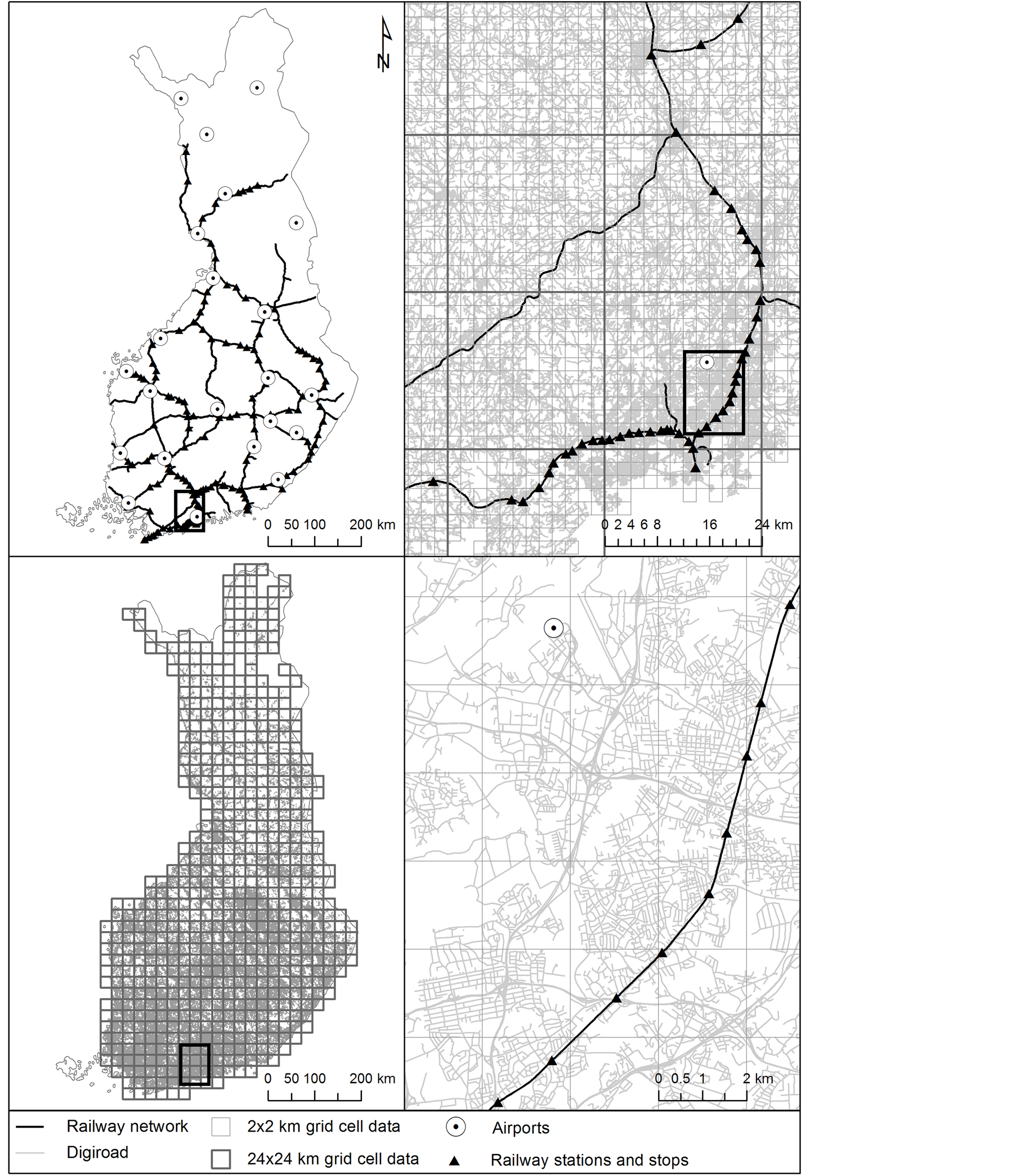
Figure 1. Illustration of grid cell, transport network and facility datasets at different scales.
negative exponential distance decay functions with the beta parameter 0.05 were also notably more explanative than the three other tested options. Thus, the empirically estimated function was selected to be used in further computations. A trend worth noting is that explained deviance is commensurate to scale for all types of potentials.
In the calculation of potential accessibility to large areas with remarkable internal gravity and differing spatial characteristics, the problem of self-potential is often encountered [55] . In regular grid cells, self-potential is commensurate mainly to population density and in this study population density is used as an explanatory variable. In addition, self-potential has little significance to potential at accurate resolution computations. Hence, self-potential was not included in potentials in this study. For the higher scales potential accessibility was calcu-
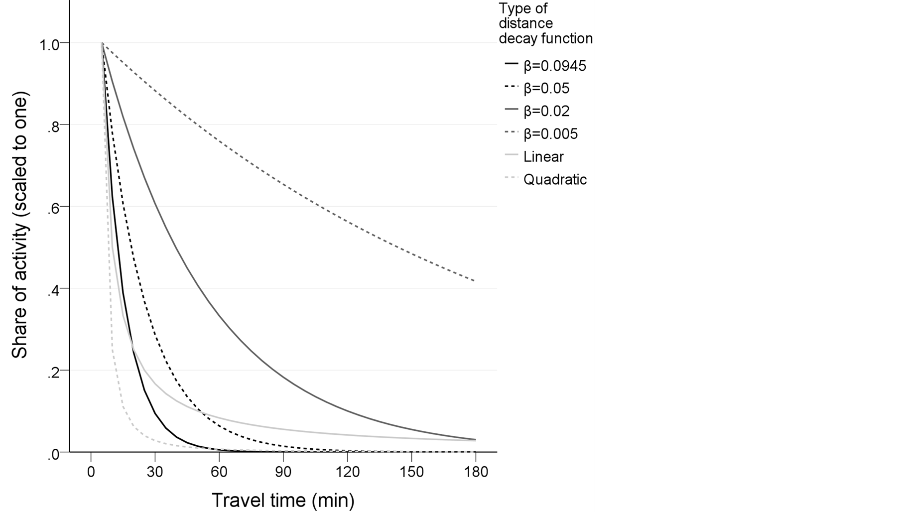
Figure 2. Form of distance decay functions.
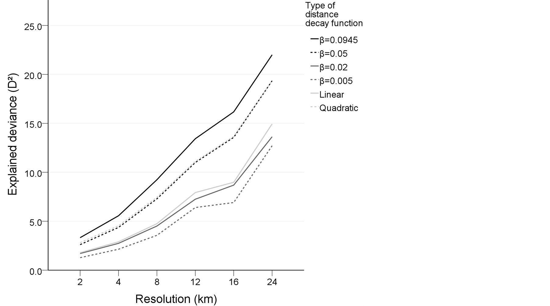
Figure 3. Explanatory power of potential accessibility by different distance decay functions.
lated as population-weighted averages of potentials at 2 km × 2 km resolution, providing a more realistic outcome than applying population-based self-potential estimates, Euclidian space-based approximations or shapebased estimates.
5.2. Airport and Railway Accessibility
Air and rail transport accessibility variables were calculated as road network-based travel times from each grid cell to the nearest airport and railway station in 2003 [56] . All twenty-two Finnish airports with scheduled flights and all 185 railway stations and stops were included in this analysis. Like in the case of potentials, accessibility was calculated at 2 km × 2 km resolution and for larger scales the population-weighted averages were used. This highly simplified approach was used to enable analysis of the effect of road-based accessibility potentials and other transport modes simultaneously in a multiple regression. For this purpose, other accessibility indicators could be applied as well. For example, multimodal accessibility potentials were considered for air and rail transports, but due to possible problems related to multicollinearity [57] , this approach had to be abandoned. A wider selection of indicators would also increase the number of statistical models remarkably. Hence, the clearest indicator, travel time, was selected.
The GIS data for airports were constructed by combining locations and usage information of airports. Also, the data for railway stations and stops were constructed by combining the information regarding usage of railway operation places with the location data. The coordinate locations were obtained by relating the linear railway kilometre locations of stations to the Finnish railway network GIS model, maintained by the Finnish Railway Administration.
6. Population and Socio-Economic Variables
Population grid databases of Statistics Finland [58] were applied to calculate the dependent variable, population change between the years 2003 and 2009, and in constructing explanatory variables representing socio-economic differences and population density in 2003. Altogether, the grid cell database consists of 108 records, including age structure, level of education, consumer structure of population, size and stage in life of households, consumer structure of households, buildings and housing, workplaces and the main type of activity of population. Observations in the database are from statistical years 2001-2003. Based on these records, an extensive set of theoretically relevant variables having a potential effect on population change was constructed. This resulted in 58 candidate socio-economic variables which were tested for their theoretical consistency and explanatory power in the preliminary analysis. Variables for each scale of analysis were built by aggregating the 1 km × 1 km data into the larger resolutions.
Due to the protection of privacy, some database records are not available in grid cells containing fewer than 10 inhabitants. The records affected by the protection of privacy include the level of education, consumer structure of the population or households, and the main type of activity of population. Consequently, the most sparsely populated grid cells had to be excluded from the analysis. The remaining data cover 91.9% of the Finnish population, but only 24.7% of inhabited 2 km × 2 km grid cells. At 2 km × 2 km resolution 10,546 cells were included in the analysis, while the corresponding number at 24 km × 24 km resolution was 516.
When potential accessibility is used to explain urbanisation, the population density variable has three roles in the statistical models. First, areas having a high population density may be attractive until the maximal land-use intensity and housing capacity are reached, which can be considered to decelerate population increase. Second, the independent variable of the study, relative population change, is dependent on the population of the grid cell. Due to this, areas with similar accessibility may have similar absolute population increase, but a different relative change because of a different base population. Thus, the population density variable controls this disparity. Third, population density works also as a control variable for potential accessibility.
7. Variable Selection Process
An extensive preliminary analysis was carried out in four stages to select variables for the final statistical models. For the first, the second and the third variable selection stage, the number of variables in each thematic class are presented. In addition to variables selected for the final models, variables excluded in the fourth stage are listed.
In the first stage of the variable selection process, the theoretical relevance of model fits and the statistical significance of three accessibility variables, 58 socio-economic variables and population density in relation to population change was analysed in the univariate context. Since variables that are found to be important at fine scales are commonly also important at more coarse scales, variables were related to population change with at 2 km × 2 km and 4 km × 4 km resolutions. In addition to testing statistical significance, the theoretical consistency of model response curves was examined before multivariate modelling. After considering the theoretical relevance and statistical significance, the most suitable 32 variables were selected for the analysis of explanatory power at all six resolutions between 2 km × 2 km and 24 km × 24 km in the second stage.
In the third stage, performance of 19 variables at multivariate statistical analyses and their mutual correlation was scrutinised. Despite the remarkable decrease in the number of variables, a majority of them were highly correlated with each other. To avoid problems related to multicollinearity in regression models, variables with the best predictive ability were selected within the groups of variables having high mutual correlations. For example, due to high similarity between the consumer structure of individuals and the consumer structure of households, the latter was excluded as it possesses lower explanatory power. The highest accepted Pearson correlation was 0.755, which was found between average incomes and share of academic education at 24 km × 24 km resolution. At stage four, 12 variables were included in multivariate models and the theoretical consistency of each variable was considered at all scales and variables were selected for the final statistical models based on this information.
The final set of variables included two accessibility and four socio-economic variables and population density. Specifications of variables are presented in Table1 The number of observations, i.e. grid cells, at each scale varies between 10,546 and 516. Although the range in observation numbers is relatively large, this is not regarded as a problem, as Kotavaara (idem.) did not find any remarkable change in explained deviance in an analysis with a small random sample and a large number of observations.
8. Results
Multivariate GAMs produced significantly stable relationships between explanatory variables and population change in relation to resolution, which is apparent in the similarities of response curves at the most accurate 2 km × 2 km and the most coarse 24 km × 24 km resolutions used in the analyses (Figure 4 and Figure 5). In addition to the characteristics of the effect, GAM fits also indicate the strength of the variable. Moreover, the effect of outliers is transparent, as observations are marked on the x-axis and 95% confidence intervals enable the consideration of the uncertainties of model fits. The main dynamics of the Finnish population are visible in the model responses. Of course, some detailed characteristics visible at the 2 km × 2 km resolution are averaged out at the 24 km × 24 km resolution. Grid cells that had increase in population are characterised by high potential accessibility, indicating that population concentrated in urban areas and in surroundings with good accessibility during the research period. The polarising effect is very strong in the centre-periphery axis, except in the urban centres where the relative growth clearly stabilises. Other variables that have an almost linear relationship to population increase at some part of the response curve describe standard of living.
Average incomes are related to population growth, except in cells with the highest incomes. Also, the high share of academic education relates strongly to population growth. As the well educated population lives mainly in urban areas, it seems that the trend of brain migration is visible in the model fit. Surprisingly, the employment rate has the weakest effect on population change at the 2 km × 2 km and the 24 km × 24 km grid cell resolutions. However, when the employment rate is 50% or lower, the model fits have very wide confidence interval, but this pertains to only 0.7% of cells at the 2 km × 2 km resolution. The population density variable relates conversely to population growth due to the high land-use intensity occurring in the densely populated areas and the disparity related to the relative population change in cells with a different number of inhabitants.
The age variable reflects clearly the natural population increase and agglomeration of young people in urban areas. However, an interesting growth trend can be found in 4.5% of the grid cells which are located on peripheries and in which the mean age is over 50. The growth in these cells occurred in proximity to the sea and lakes, whereas inland cells experienced a drastic reduction in population. Whether this trend can be associated with such processes as remigration or rural second housing is a question demanding further study.
Performance of models was investigated in relation to resolution in terms of explained deviance (D2) and predictive ability (Figure 6). To assess the difference between non-linear and linear modelling framework, regressions established also with GLM. Based on these figures, the explanatory power and predictive ability of models are almost directly proportional to the resolution of grid data. This trend pertains also to performance of GLMs, which have almost as good explanatory power as GAMs in coarse resolutions. However, the relative difference in explanatory power between non-linear and linear models is high at accurate resolutions. Similarity between correlations based on all observations and cross validation refers to consistency of models. Multivariate models at 24 km × 24 km resolution have a good predictive ability on population change, as the correlation between population change and predictions is about 0.8 with four times cross validation and also with a full dataset. At 2

Table 1 . List of dependent and explanatory variables selected for the final statistical models.
km × 2 km the predictive ability of a model is moderate as models resulted in correlations which are near to 0.4. However, a visual comparison between population change and model estimates shows that the model at 2 km × 2 km resolution captures well the main trends of population change in geographic space (Figure 7). At univariate models, explanatory power of each particular variable increases along with resolution, and the explanatory performance of potential accessibility is the highest of all variables at all resolutions (Figure 8). Incomes and share of academic education explain population change nearly as efficiently. Mean age, employment rate and population density explain population change at a tolerable level. It is interesting to noting that population density, a common variable related to analysis of urban areas, has the lowest explanatory power at accurate resolutions.
In addition to considering the explanatory potential of each variable in univariate models, the importance of each variable in relation to other variables in multivariate models was tested by drop contribution. Drop contributions are obtained by dropping each explanatory variable from the model and by calculating the associated change in deviance. In other words, variables having a high drop contribution can explain a considerable amount of deviance that other variables are unable to explain. According to drop contributions (Figure 9), potential accessibility has the most essential complementary role in multivariate models at resolutions more accurate than 16 km × 16 km. Only at largest resolutions the age variable has a slightly more important role. Also, a trend worth mentioning is the low importance of academic education at the largest scales, which indicates that the relationship between population change and the deviation of education occurs at local or sub-regional scale. The low importance of employment rate in explaining population change is probably connected to high level of social security in Finland.
9. Discussion
The results of this study show that with a careful selection of accessibility and socio-economic variables, population change can be modelled tolerably at accurate resolutions and well at coarse resolutions. The explanatory power of the models, particularly at accurate resolutions, relies greatly on potential accessibility, a ratio expressing geographical distribution of transport infrastructure capacity and population. This relationship indicates the strong influence of scale economies on Finnish population change, in which the major trend of urbanisation did not begin until the 1960s. It is also interesting that population density is much weaker in capturing population change in comparison to potential accessibility. On the basis of this, it may be reasonable to include accessibility in the quantitative definitions of urban areas, instead of population densities alone. Also socio-economic differences have, of course, a strong relationship with population change. It seems that population growth occurs in areas with high overall education levels, incomes and employment, whereas a high average age is usually as-
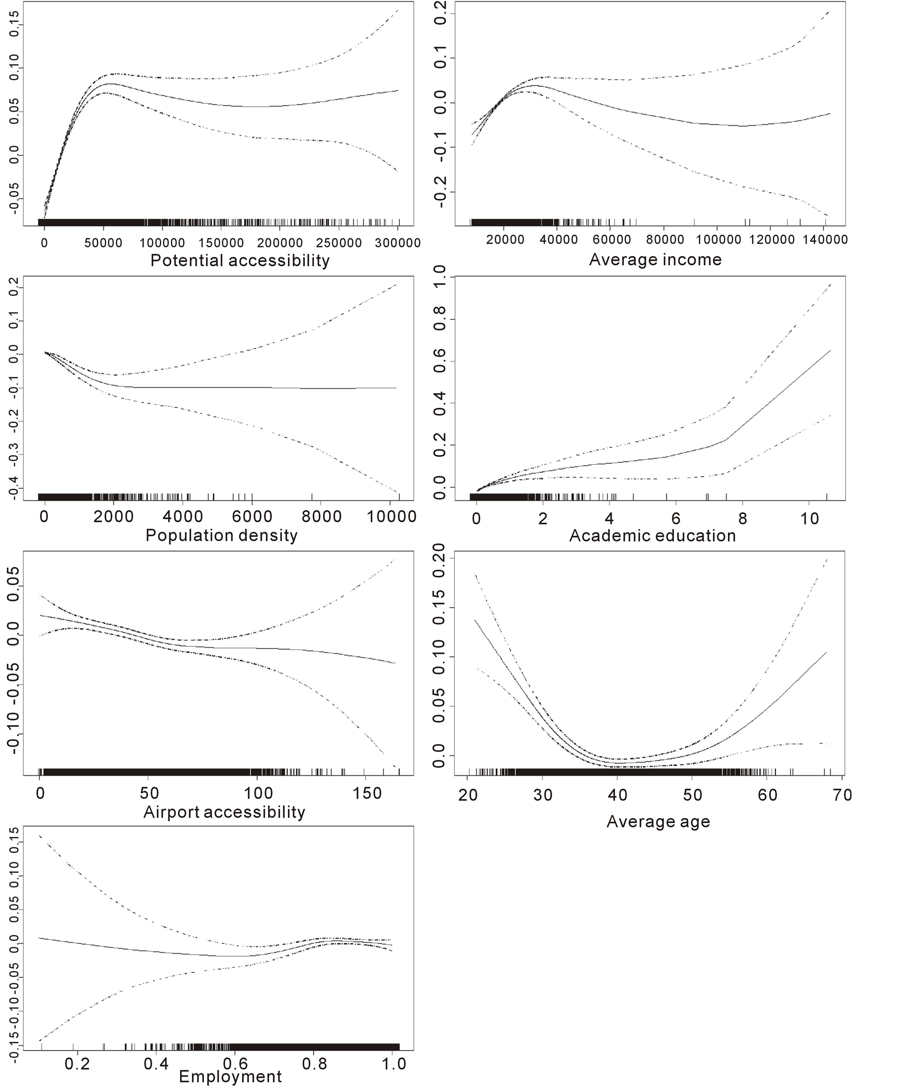
Figure 4. 2 km × 2 km grid cell multivariate model response curves. The vertical axis represents the effect of the variables on logarithmic population change. Tick marks show the location of each observation along the value range of the variable. The confidence interval of 95% is presented with a dashed line.
sociated with decreasing population. Accessibility of airports has a clear growth effect on population. Considering this, it is interesting that the railway accessibility variable had to be ignored due to inconsistency and low statistical significance.
With regard to the distance decay function used in the calculation of potentials, the relatively steep, empirically estimated function turned out to be the best of all the tested options. A possible explanation for the success of this function is the accurate scales assessed in the study. In contrast to using administrative regions in the
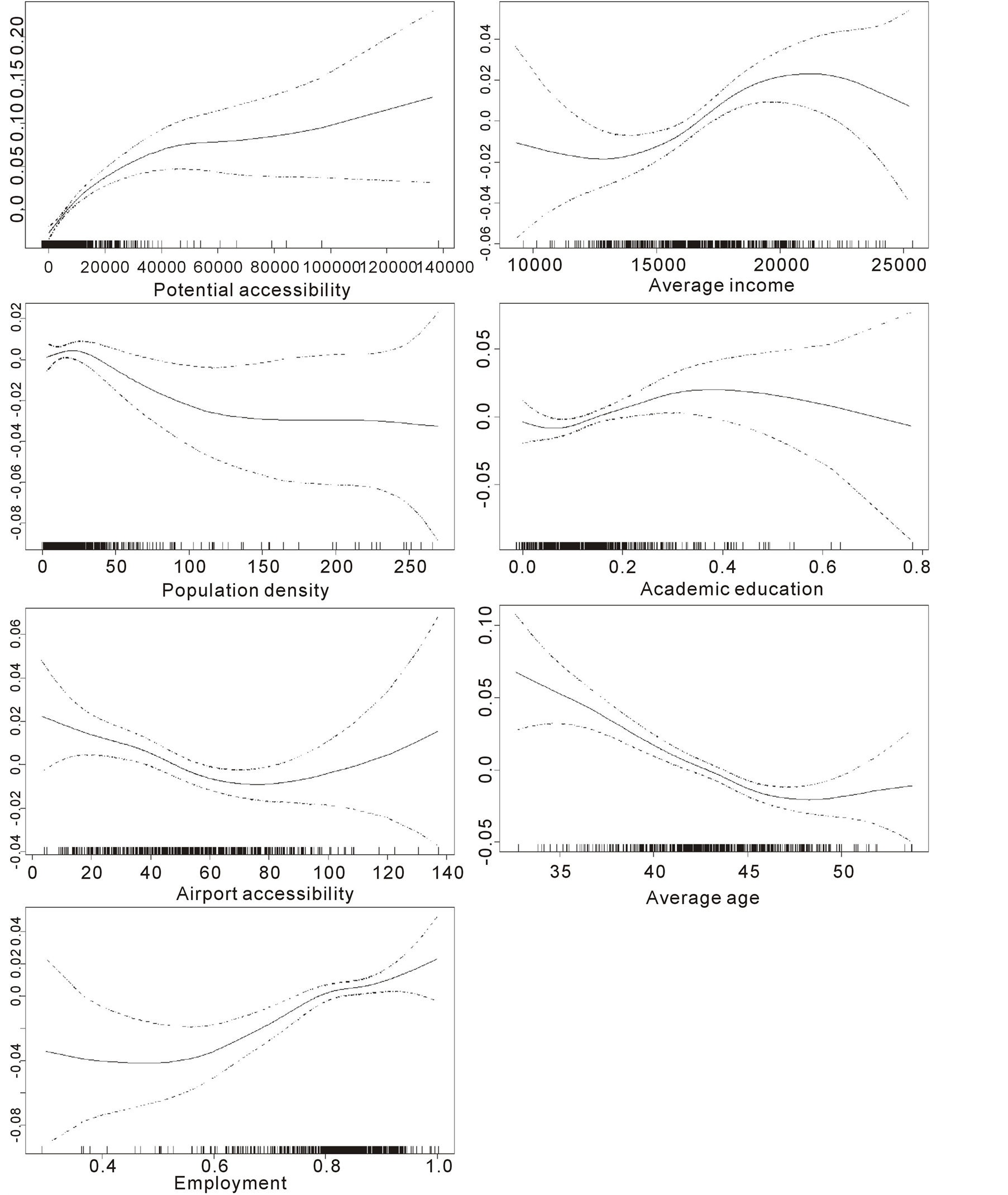
Figure 5. 24 km × 24 km grid cell multivariate model response curves. The vertical axis represents the effect of the variables on logarithmic population change. Tick marks show the location of each observation along the value range of the variable. The confidence interval of 95% is presented with a dashed line.
calculation of potential accessibility, requiring the use of internal distance estimates and self-potential, high resolution grids make it possible to detect short-distance patterns. Thus, it is advisable use this study’s beta parameter with accurate resolutions, however great care must be taken when applying it to larger scales.
Regressions are usually based on linear response shapes and non-linear relationships are analysed through transformations. Although the established models produced response curves that were mostly positive or negative, they only partly follow the linear form. When the statistical models are established in the linear framework
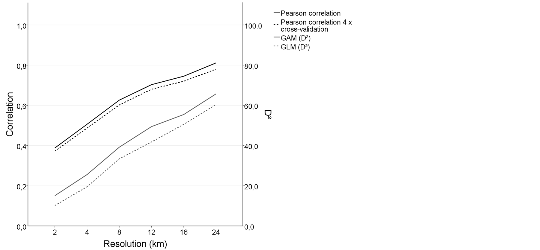
Figure 6. Performance of GAMs and GLMs (D2) in explaining population change in relation to resolution. GAM validation with Pearson correlation is presented by applying four times cross validation and validating predictions for the full dataset including all observations.
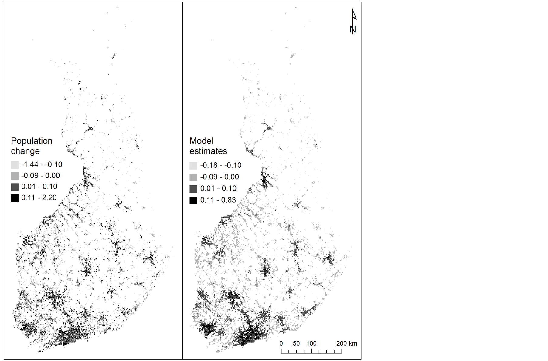
Figure 7. Population change and model estimates between 2003-2009 at 2 km × 2 km resolution.
the characteristics of the relationships are not as precise, and explanatory power is harmed, particularly in the case of accurate resolutions. Therefore, there are clear benefits in establishing the relationships in explorative analysis in non-linear form.
The results of this study also need to be considered in the light of classical problems, the modifiable areal unit
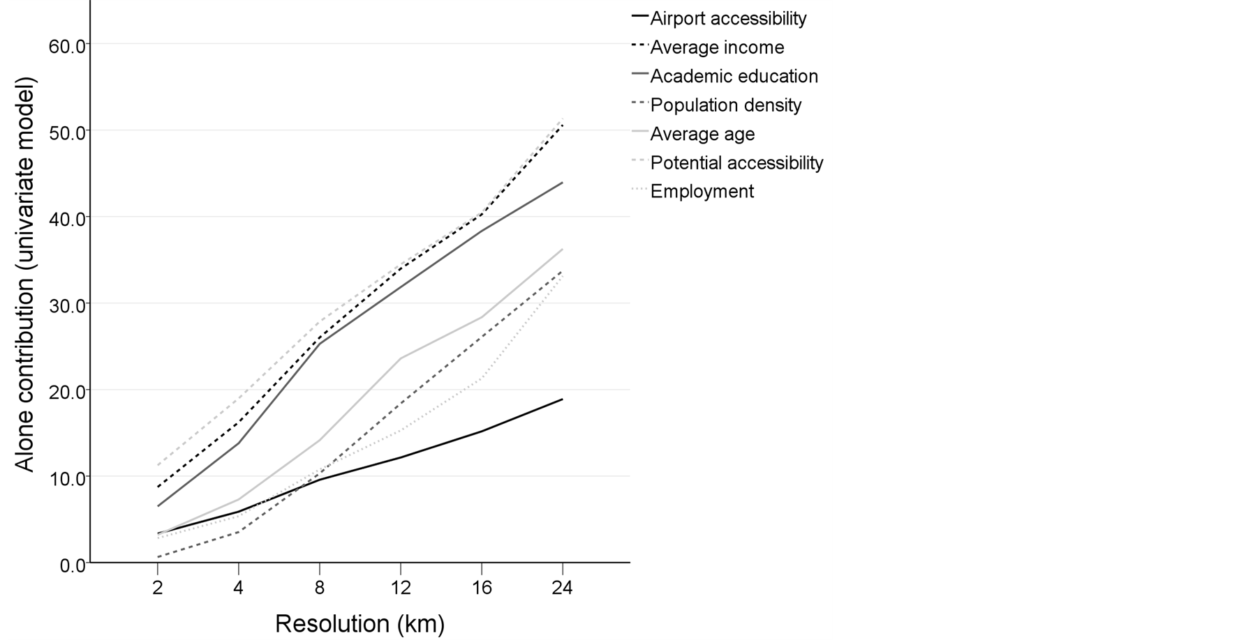
Figure 8. Performance of each variable as alone contribution (i.e. explained deviance of univariate models), presented in relation to resolution.
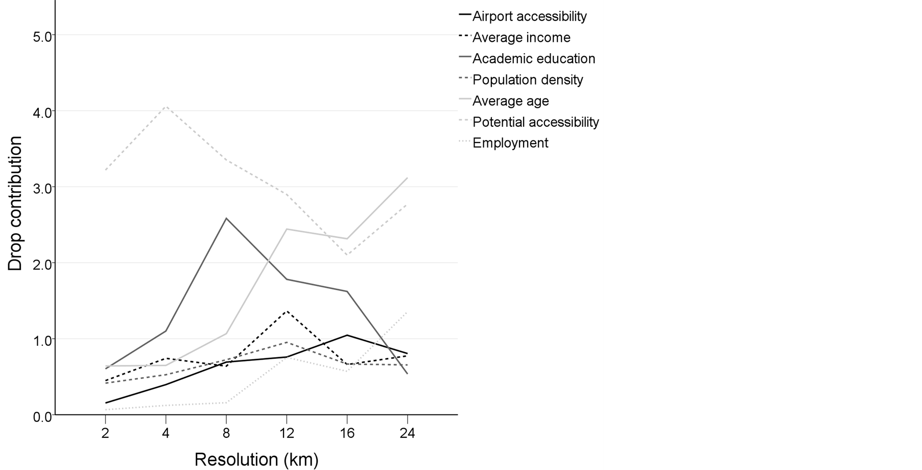
Figure 9. Performance of each variable as alone contribution (i.e. explained deviance of univariate models), presented in relation to resolution.
problem and ecological fallacy, see for example [59] . It is definitely an important finding that models with selected variables produced consistent fits at different scales. Hence, a classical problem related to modifiable areal units, does not seem to pertain to the relationships established for the resolutions of this study. However, another classical problem, ecological fallacy, needs to be taken into account seriously. The explanatory power and predictive ability of models decreases strongly when the scale of the analysis becomes more accurate. Correspondingly, results of the study cannot to be extrapolated to resolutions more accurate than those analysed, and particularly not to the individual level.
Spatial autocorrelation is also an important issue for discussion. Some spatial autocorrelation exists inevitably in any population data consisting of small areal units. According to Andersson and Gråsjö [60] , in regression models representing trends in a society connected by transport networks, accessibility variables may be operationalised to models with a motivation to reveal spatial dependencies. Furthermore they state that, significance of the spatially discounted variables can be interpreted as spatial dependence, the presence of any kind of spatial dependence can invalidate regression results, and consequently, the autocorrelation cannot be ignored. However, their model shows that spatial dependence in the error terms vanishes when the model includes accessibility variables and, if accessibility variables are statistically significant, it suggests that problems of spatial autocorrelation are significantly reduced.
The data used in the study admittedly involve certain issues that may affect the results. Due to protection of privacy of individuals, 1 km × 1 km grid cells with small populations are not available for research use. Thus, a relatively large proportion of deep peripheries was inevitably excluded from the models. The analysis covered 91.9% of the population, but only 24.7% of inhabited 2 km × 2 km grid cells. The distance decay function applied to the potential accessibility variable was defined on the basis of a regional traffic survey. The characteristics of the function may possibly be somewhat different, and its reliability improved, if a national traffic survey or other equally extensive regional traffic surveys had been available. Potential accessibility is based on the idea of gravity and travel densities, but the sphere of living and the matter of distance are, in the end, very specific to the individual. Supply and demand of transport are not homogenous and multi-modal travel chains are common. Hence, distance decay functions should be refined more specifically in relation to an area, a phenomenon and socio-economic characteristics.
10. Conclusions
Since population change in Finland has previously been statistically assessed mainly through the municipal division, assessment based on grid cells improves the spatial accuracy remarkably. Furthermore, this study is a tentative, but novel attempt to carry out small area predictions of populations. This can be considered to be particularly important for spatial planning, including the location planning of services and business activities, and more generally for policy making, because a majority of investments are made in the long term, rather than for the present situation. The validation of the statistical models proved that they are consistent enough to be extrapolated, if the characteristics of population dynamics remain the same in space or time. As the predictions are based on smooth functions, the conditions existing in the prediction variable set must also be characteristic of the calibration data. The presented statistical models indicate that it is also possible to attain an analytical compromise between the spatial resolution and predictive power in the modelling of population change, and multi-scalar modelling procedure is an applicable approach for this. However, in order to apply the prediction directly in planning, more research is definitely needed to increase the predictive ability.
The results of this paper outline the characteristics of Finnish population dynamics, and also raise some pragmatic policy-orientated questions. As it seems, road based accessibility mainly benefits the centre areas, and therefore it would be possible to ask whether it is useful to direct the cohesion policies on road infrastructure issues as long as a decent level of transport networks are available in most areas? Another interesting question concerns the role of airports. The proximity of airports seems to attract a population, which probably results from indirect location choices of companies and the associated positive effect on employment and migration. Therefore, airports are clearly important for regional development in Finland. However, regardless of a remarkable rationalisation of railway transports during recent decades and a vast decrease in the number peripheral stations, similar growth pattern could not be related to railway accessibility. When this notion is combined with the urban sprawl trend, it can be concluded that the opportunities to improve public transports at the local level by railways in the future may be lost, and the sprawl trend in general will impair opportunities to develop a more efficient public transport system.
Even though the modelling results of the study are very country specific, the scale dependency in population dynamics may prove to be a common trend. Moreover, empirical-statistical modelling procedure may be applied to scrutinise also other areas, provided that data on infrastructure, population and socio-economic conditions are available at a reasonably fine resolution. Finally, the most critical argument based on this study is that there is an evident need to bring accessibility to the core of small area population change models.
Acknowledgements
We wish to thank the ESPON TRACC project and particularly Klaus Spiekermann for discussions about accessibility and regional development as well as two anonymous referees for their perceptive comments that helped improve this paper remarkably. Also the valuable comments of Heidi Määttä-Juntunen, Mikko Tervo and Tiina Lankila are acknowledged, as well as the work by Ari Nikula on constructing the railway database used in this study. The analyses for the paper were based on the methodological work carried out during the project “Finnish Railways in the Nordic and Russian context (FiRa)”, which was funded by the Academy of Finland. FiRa was a cooperative sub-project of the European Science Foundation’s (ESF) project “The Development of European Waterways, Road and Rail Infrastructures: A Geographical Information System for the History of European Integration (1825-2005)”. The work for this paper was funded by The Department of Geography at the University of Oulu, the Geography Graduate School, the Foundation of Science at Oulu University Scholarship Foundation, the Foundation of Tauno Tönning and the Foundation of Emil Aaltonen.