Validity of Approach to Maximize the ASR of the Order Superiorly Two in Discrete Nonlinear Systems ()
1. Introduction
It is widely believed that in the field of automation, several constraints of physical nature have an effect on the dynamic behavior of non-linear systems. Consequently, the study of a system-dynamics comprises a preliminary and important phase so that we can find out about the strategy of a powerful and reliable order. Obviously, the study and analysis of the stability of dynamic systems involves an essential stage for any resourceful study. Thus, the concept of asymptotic stability of autonomous continuous systems is elaborated today. In 19th century, this notion came into existence with the theory of Lyapunov in an attempt to create an interest-center to a huge number of research-works and research-works; in this, the theory of Zubov [1] -[3] is a case in point. Such a theory, in fact, provides a common scope for study of all the nonlinear autonomous continuous systems. Hence, the two following issues are regarded as major problems:
• The analysis of the stability of nonlinear dynamic systems.
• The estimate of a relatively exact region of the state-space ensuring the stability of nonlinear-system variables.
When we are inclined to the study of stability in continuous time, we can perceive the richness of the literature which is teeming with results, methods and approaches dealing with these themes [4] -[6] .
Nevertheless, when dealing with the problems of analysis and stability of the discrete autonomous nonlinear systems, we note that a few works address such problems [7] -[10] .
In this, this article is aimed to study the stability and to determine a field of stability of the discrete autonomous nonlinear dynamic systems.
We also realize that most of the studies dealing with this subject are based on the Lyapunov theory. We insist on the fact that, for a nonlinear system, the determination of an asymptotic stability region around an equilibrium point is generally a hard task. Again, we are appealed to the synthesis of a numerical technique so as to analyze the asymptotic stability in the neighborhood of the discrete systems stable equilibrium points.
This approach is developed in other works [11] -[13] . Its principle aims at executing in the opposite directions of the iterations described by the recurring polynomial state equation. Such equation represents the dynamics of the studied autonomous discrete nonlinear systems. The reverse discrete system, then, will be characterized by the same samples belonging to the closed curves in the state space and which represent the same dynamics of the initial system. But its discrete direction of evolution is quite the reverse. Consequently, the origin becomes unstable and the speed of the closed curves connecting the discrete points initialized in an asymptotic stability field is reduced. This, in fact, allows identifying a broader stability region.
Indeed, the reverse trajectory method paves us the way to reach the exact field of asymptotic stability of the nonlinear discrete systems of order 2. Nevertheless, it is applied to the systems of an order equal to or higher than 3 in orders to widen the initial field of stability without reaching the exact field of stability.
This paper is organized as follows: in the first section.
2. The Discretization Method
The method of studying a discrete process looks like a transposition of the methods which are initially developed for the continuous systems. This actually pushes us to study the analogy between the continuous and discrete process which paves us the way to use the numerical and analogue methods by control and simulation.
In this part, we are inclined to the determination of a discrete model of the continuous systems.
Initially, we consider the continuous model defined by the following equation:
 (1)
(1)
We employ the continuous model of order three which is defined by:
 (2)
(2)
By considering a discretization period T, which is properly selected and by adopting the following approximations in an interval :
:
Let us consider, then, the following discretization method [14] [15] :
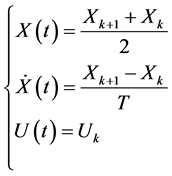 (3)
(3)
By including Equation (3) in Equation (2), here comes the discrete model given by:
 (4)
(4)
where

3. Linearizing Polynomial Control of the Discrete Nonlinear Systems
3.1. Description of the Studied Discrete Nonlinear Systems
The concept of the discrete NLGS approach is derived from the same methodology as the continuous NLGS one. In addition, we discredited the continuous model so as to simplify the analysis and to facilitate the task of associated calculation [16] . The discretization of continuous systems is particularly significant today as the current technology requires the implementation of discrete controls [17] .
The studied discrete nonlinear systems are defined by the state equations of the form [18] [19] :
 (5)
(5)
where  is the state vector
 ,
,  is the control vector
 , the functions
  and
and  are assumed to be analytical.
Let us consider the following variable change , where the operating point state vector is
  and
and  is the corresponding control input. Using the development into generalized Taylor series expansions and the kronecker tensorial product given by:
 (6)
(6)
3.2. The Suggested Approach to the Control
3.2.1. Formulation of the Problem of Linearizing Control
Let us consider the discrete nonlinear system (1) and consider an arbitrary linear system of order n described by the following state equation [7] -[20] :
 (7)
(7)
It is a question of determining, when there exists, a nonlinear feedback of the form:
 (8)
(8)
Here is a nonlinear analytical transformation described by the following equation:
 (9)
(9)
Such that (5) is transformed into the linear system (7).
3.2.2. The Control Determination
By using the polynomial development of the functions  and
and , the relations (8) and (9) are written as:
 (10)
(10)
where  is the redundant power.
The control vector  and the state analytic transformation are defined by the matrices
  and
and .
.
By replacing the functions  and
and  with the developments (6) in the state Equation (5), we can get:
 (11)
(11)
After replacing the control vector  with the development (10), Equation (11) becomes:
 (12)
(12)
Such equation can be stated in this form:
 (13)
(13)
where 
The vector defined in Equation (9) verified:
 (14)
(14)
and for 
 (15)
(15)
where
 (16)
(16)
In particular, we have
 (17)
(17)
and
 (18)
(18)
The expression (14) truncated to the r order:
Using the polynomial development functions  and
and , the relations (7) and (10) are written as:
 (19)
(19)
other
 (20)
(20)
By replacing  which is defined by System (7) in Equation (10), we obtain the form:
 (21)
(21)
where  is a redundant matrix.
The identification of the relations (20) and (21) leads to the following recurring equations:
 (22)
(22)
The choice of the matrix  such as
  implies:
 (23)
(23)
when the function  is introduced into the Sylvester Equation, it comes [21] :
 (24)
(24)
where
A necessary condition of existence of the matrix  and the matrix
  itself is a full row. When this condition is satisfied, the relation (24) leads to what may be said as satisfied:
 (25)
(25)
where
 is the pseudo-inverse of
 .
.
Equation (25) allows for the determination of the coefficients of the matrices . The parameters
  of the control law are selected such that the standard
  is minimal. This minimization leads to the following expression of the matrices
 :
:
 (26)
(26)
4. The Principe of the Algebraic Inversion of the Recurring State Equation
This principle derives its effectiveness from the fact that the asymptotic speeds of the points belonging to the closed curves (when ) constitute an integral part of the border of the searched stability region. This technique is identical to that developed in the case of continuous systems.
This method is obviously based on the execution of the iterations by reversing the sampling moments described by the parameter k of the state Equation (13) and represent the autonomous nonlinear discrete polynomial system [22] -[25] . Likewise, we have to consider the system described by the following equation:
 (27)
(27)
Such a system is called reverse, it is characterized by the same samples belonging to the closed curves of the state space and which describe the discrete dynamics of the system (13) but by reversing the direction of the states. The origin which is thought to be stable for the system (27), thus, becomes unstable for the system known as reverse (13).
5. Algebraic Approach to the Inversion of the State Discrete Equation
This section is dedicated to the synthesis of the analytical methods which aim at approximating the recurring state equation of the studied discrete system through a state equation which describes its evolution in the opposite direction in the state space.
An algebraic approach will then be considered [26] . Such an approach considers an initial field of asymptotic stability around an equilibrium point to carry out, thereafter, converse iterations allowing us to widen the initial field of the considered stability.
Let us suppose then:
 (28)
(28)
This assumption is rigorously justified in the case where the evolution from iteration to another is done with an optimal choice of the sampling period.
According to the analytical development given in [22] , we assume in the remaining part of this paper that the classes of discrete systems under consideration are truncated to the third order which can be written as follows:
 (29)
(29)
By replacing  by its expression (29) in (28) and by neglecting the terms
 , for
, for , we can easily reach, after identification, the following equality:
 (30)
(30)
where

The expression (30) characterizes the term  which describes a weak variation of the deviations describing the dynamics of the models studied between two successive sampling moments. The representation of the discrete state (28) is regarded as an approximation of the dynamic behavior in the reverse direction of the studied systems discrete states. Such an approximation is, in fact, an assumption which will be as much satisfied as the variation
  is reduced. This imposes the choice of a weak sampling period [26] [27] .
6. Synthesis and Implementation of an Algorithm of Estimating an Attraction Domain
In this section, we suggest a synthesis algorithm which allows formulating the principal steps leading to the estimate of an asymptotic stability region of the discrete nonlinear systems [24] . Thus, the estimated ASR can be arbitrarily approximated by means of sequence of convergence of simple successive fields generated by Equation (13). Firstly, we start with an Initial Region of Asymptotic Stability (IRAS) noted by . A new field is, then, obtained by applying the first iteration of (13).
This algorithm is presented in 4 steps:
Step 1: It tends to determine the system equilibrium points out of the original point and to analyze the local stability of each point.
Step 2: It is likely to determine an IRAS  in the space around each asymptotically stable equilibrium point.
Step 3: It concerns the development of an iterative calculation based on Equation (13) initialized by a departure stability field  determined in Step 2.
Step 4: It consists in stopping the iterative calculation based on Equation (13) when a broad ASR is obtained after the convergence of the curve towards a limited form.
The application of Step 1 does not generally present any difficulty, contrary to the determination of a IRAS. In order to solve this problem, we used a technique presented in [22] [23] .
The detailed analysis of the algorithm allows us to deduce some remarks and conclusions similar to the case of the reverse trajectory method considered for the continuous systems. Actually, the topological and graphic character on which this algorithm is based shows some difficulties for the high order systems. Nevertheless, it remains effective for reduced order systems .
.
• Concerning the second order systems, the method converges towards a sufficiently large asymptotic stability region in a minimal time. This result comprises a very important performance in the context of synthesizing control laws that will be established on line [28] .
• For the systems of order higher than two, the method remains also applicable only to widen the initial asymptotic stability region. A sufficient number of  reverse iterations allows obtaining a border
  which limits a larger domain of asymptotic stability
 .
.
Theorem [25] :
The discrete time state variables of Equation (13) are exponentially stable in the ball , where
  is the positive solution of the polynomial equation:
 (31)
(31)
where  are positive numbers verifying:

7. Simulation Results
The problem of transitory stability of the generator-systems becomes increasingly important because of the remarkable increase in the network dimensions of production and the transport of electrical energy [29] [30] .
It is perceived that the stability of the production systems of electrical energy is never global but local around an operating state considered as an equilibrium state.
This typical problem brought about by the disturbances in the production systems stability is the main factor that encouraged us to consider the exact asymptotic stability region of the considered systems [31] [32] .
The very study is about the application of the method of the suggested approaches to the linearizing control of a synchronous generator.
The synchronous generator can be described by a model of order three characterized by the state vector [33] :
 (32)
(32)
As for input, it has the excitation tension .
.
The following Equations represent this model [34] :
 (33)
(33)
where  is an additional component which is expected to improve the performance of the small-scale model of the generator, and
  for
for  are the constants given by:

The development of the Equations around an operating point  leads to the following polynomial non-linear model [35] :
 (34)
(34)
where
 (35)
(35)
The studied generator is characterized by the parameters expressed in the following reduced values (per unit “p.u”) [34] :

The discretization of the continuous model of the synchronous generator leads to a polynomial model of the following form:
 (36)
(36)
with:

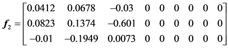

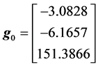
The application of the control approach to the obtained discrete model lets us determine a polynomial control law:
 (37)
(37)
And a non-linear transformation
 (38)
(38)
The line matrix  is, in fact, selected in a way that the dynamics of the arbitrary linear system is defined by poles equal to 0.6, 0.7, 0.7 which yield:

The line matrices  and
and  are given by:


The validation of this nonlinear control law is yielded by simulation. The curves represented on Figure 1 to Figure 4 illustrate the regulation conditions of the variables ,
,  ,
, . On these curves, in fact, one can perceive an obvious improvement of the performances of the processes, especially from the point of view of the decrease of the oscillatory mode and the speed of the convergence of the different variables of the machine. These good performances are obtained with the help of a control signal. This control signal evolution is actually suitable and satisfactory.
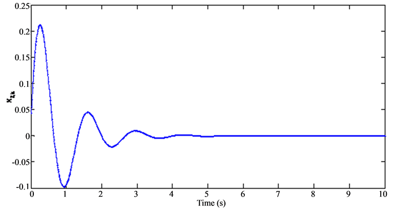
Figure 2. Evolution of the state .
.

Figure 3. Evolution of the state .
.

Figure 5. Aymptotic stability region of two Axes.
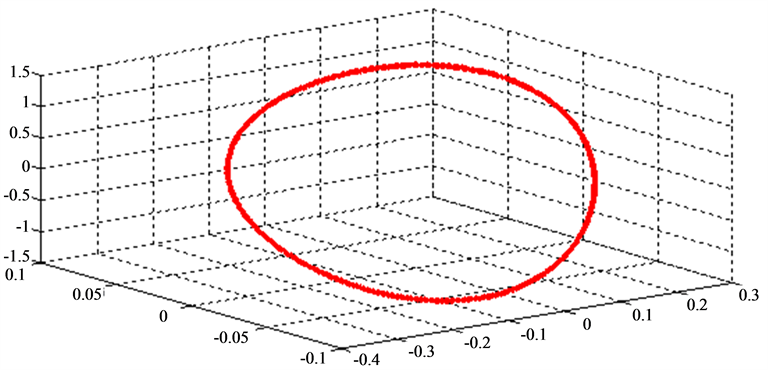
Figure 6. Asymptotic stability region of the synchronous generator.
Indeed, we may notice that the variables quickly return to the origin and that the recorded excesses remain within the tolerated limits. The same conclusion can be drawn to the control signal which permits to ensure this powerful regulation.
The discrete Reverse Trajectory Method (RTM) is theoretically exploitable for any locally stable nonlinear system. Moreover, it proves its effectiveness through the advantage of being numerically implementable for high order systems. What is more, one may also note that the performance of this method largely depends on the determination of an asymptotic initial region which will be used as an initial field for integration in opposite direction. We apply RTM so as to determine an Asymptotic Stability Region (ASR). The results of this step are given in Figure 5 and Figure 6.
We notice, in Figure 5 and Figure 6, the method remains applicable to the systems of order higher than two.