Simplex Optimization and Its Applicability for Solving Analytical Problems ()
1. Introduction
Simplex is a geometric figure, formed on the basis of  points
  in the n-dimensional space, i.e., a number of the points exceeds the dimension of the space by one. These points are referred to as the vertices of the simplex. Distribution of the points
  in this space is represented by a matrix of this simplex. Specifying the coordinates for
  is easy if it concerns the
  or
or  space, but it becomes less comprehensible when the issue concerns the n-dimensional
  simplex. Although in the literature [1] one can find ready-made forms of the simplex matrix in
  space, but information on how to receive it in an easy manner is lacking.
The simplex concept is the basis for the Nelder-Mead [2] simplex optimization procedure (SOP) [3] , conceived as a modification of the simplex method of Spendley, Hext and Himsworth [4] . The SOP is easy to use, and does not require calculation of derivatives [5] [6] , as in the gradient (local steepest descent) method [7] [8] ). The SOP is widely applicable and popular in different fields of chemistry, chemical engineering, and medicine [9] . Furthermore, it works well in practice on a wide variety of problems, where real-valued minimization functions with scalar variables are applied.
The sequential simplex method is considered as one of the most effective and robust methods applied in methodology of Evolutionary Operation (EVOP) experimental design [10] -[15] . The SOP method was implemented in MINUIT (a Fortran from CERN [16] package), then in Pascal, Modula-2, Visual Basic, and  [17] . The iterations are stopped when the function minimized is less than a preset value.
In this article, the problem of obtaining the simplex matrix in  space will be presented on the basis of the triangle and the scalar product concept, well-known to the students from earlier stages of education. The evolution of the simplex according to SOP [3] [18] will also be presented in a understandable manner.
2. Simplexes in 2-D and 3-D Space
In order to introduce the simplex concept, we start from the point , (I) segment
 , (II) equilateral triangle
 , and (III) tetrahedron
  concepts, known from the elementary geometry. The
 ,
,  ,
,  ,
,  (and generally
 ) notations express the dimensionality of the corresponding geometrical entities (Figure 1).
The points: ,
,  ,
,  are vertices of the triangle
 ; the points:
 ,
,  ,
,  ,
,  are the vertices of the tetrahedron
 .
.  is one of the edges of the triangle;
  is one of the edges of the tetrahedron. Equilateral triangle
  is one of walls of the tetrahedron.
Segment, equilateral triangle, and tetrahedron can be presented in the same scale; it means that all distances, equal to unity (chosen arbitrarily), between the (neighbouring) points  and
and  of a polygon are assumed, i.e. the length
 .
.
All angles between edges of the equilateral triangle are equal to 60˚ . All angles between adjacent tetrahedron edges are equal 60˚ too, owing to the fact that all the tetrahedron walls are composed of equilateral triangles
 . By turns, tetrahedrons form the
  walls in
  polygon, etc. It means that all angles between adjacent edges of a symmetrical
  polygon are equal 60˚, as well.
The equilateral triangle can assume different positions on the plane. A particular case is the triangle with unit edges, “anchored” at the origin of co-ordinate axis, as one presented in Figure 2.
The successive vertices of the equilateral triangle can be presented in matrix form, where the rows are expressed by co-ordinates of the corresponding points :
:
 (1)
(1)
The second and third rows of this matrix are identical with components of transposed vectors:  and
and , respectively:

The tetrahedron can assume different positions in  space. A particular case is the tetrahedron anchored at the origin of co-ordinate axis as one presented in Figure 3.
The successive vertices of the tetrahedron can be presented in the matrix form:
 (2)
(2)
The second, third and fourth rows of this matrix are identical with components of the transposed vectors: ,
,  and
and , respectively:

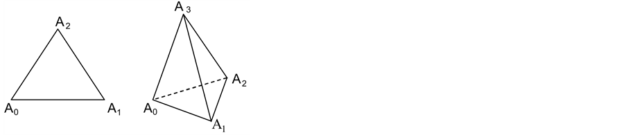
Figure 1. Equilateral triangle and tetrahedron.
3. Simplexes in n-D Space
The segment, equilateral triangle and tetrahedron are imaginable concepts. However, application of the concepts involved with geometric figures of higher dimension  is beyond imagination. One should be taken into account that, in the simplex optimization, we are forced, as a rule, to consider higher number of factors influencing the optimizing process.
Although the figures in  space (Cartesian co-ordinate system) are beyond imagination, one can present them in projective space. In Figure 4, any pair of points of the simplex is connected, informally, by a segment (line); the segments (sides, edges) are marked there with broken lines. Particularly, two points form the
  simplex in
  space. Adding a third point (that not lies along the segment or its extension) gives a triangle (
 simplex) in
  space. Adding a fourth point in
  space (not coplanar with
  simplex plane), one obtains a tetrahedron (
 simplex), etc. Generally, adding a successive
  -th
-th  point, do not lying in surface formed by
  simplex, one obtains the
  simplex. In other words, adding the successive point that not lies on (or in plane of) simplexes of lower dimension and connecting it, every time, with the remaining points, one can imagine the simplexes with larger and larger dimensions, in projective space.
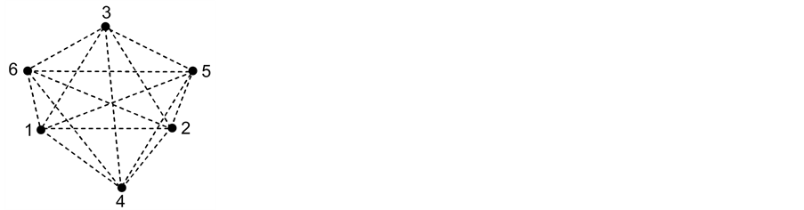
Figure 4. Formation of consecutive dimensions (up to ) of a simplex in projective space.
Let us assume that the polygon is “anchored” in n-D-space in such a manner that  is in the origin of the co-ordinate axis and any successive point “enters” the new dimension of the n-D-space, see Figure 4. It means that the co-ordinates of the corresponding points of
  polygon are as follows:
 (3)
(3)
This means that  for
for .
.
As stated above, the number of vertices exceeds, by 1, the dimension of the space; it means that the polygon in  space involves
  vertices.
We consider a pencil of n unit vectors,  , all starting from the point
 , i.e., origin of co-ordinates of
  space and ending at the points
 . One should notice that the basic components
  of the vector
  starting at the origin of co-ordinates, are identical with co-ordinates of the point
 . Then for the vectors
  based on the points specified in (3) we have:
 (4)
(4)
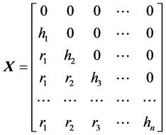
Let us construct the matrix  (Equation (5)) composed of the co-ordinates of the corresponding points in
  space:
 (5)
(5)
Moreover, we assume non-negative values for the coordinates, i.e. , and then the elements of the matrix
  can be specified as follows:
 (6)
(6)
Let  be the unit vector along the i-th axis, Xi, i.e.
 . The
. The  vectors form a set of mutually orthogonal vectors in
  space. The scalar products:
 (7)
(7)
where  is the Kronecker symbol.
Any vector  in
in  space can be also written as
 ;
;  . Then the scalar product of two vectors,
  and
and , in
, in  space is as follows:
 (8)
(8)
where  is the angle between vectors
  and
and  spanning the simplex in
  space. The angle between different vectors
  and
and  of
of  simplex equals
  [rd], i.e.
and then , for any pair of the vectors
  and
and : in triangle
 , in tetrahedron
 . Moreover,
  and then
 . If the unit vectors
are assumed, i.e.,  , then from (8) and (4)-(6) we have:
 (9)
(9)
 (10)
(10)
From (9), (10) and (6) we get, by turns,

 , i.e.


and so forth. On this basis, one can write:
 (11)
(11)
 (12)
(12)
The elements  of the matrix
  (Equation (5)) are thus derived with use of principles of elementary algebra and geometry. Then the
  simplex can be written in the form
 (13)
(13)
One can notice that hj (Equation (15)) is the height of  symmetrical simplex and
  (Equation (16)) is the radius of
  sphere (for
 —circle, for
 —“normal” sphere) inscribed in
  simplex. Moreover, we have the relations:
 (14)
(14)
where Rj is the radius of  sphere circumscribed on
  simplex, see Figure 5.
In particular, for , the matrix
  (Equation (13)) has 7 columns and 8 rows.
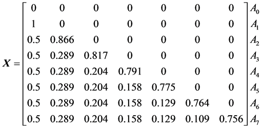 (15)
(15)
4. Translation and Reflection of the Simplex
A simplex can be translated and/or rotated in space. Particularly, the simplex defined by  (Equation (13))with the centre at
 , can be parallely shifted to the centre
  of the co-ordinate system. This way, one obtains a new matrix
 (16)
(16)
with  and
and  as ones in Equations (11), (12) and (14). Reflection of particular vertices of the matrix
  in the centre of co-ordinate system
  gives the simplex described by the matrix
 (17)
(17)
where —identity matrix.
The positions of the simplex presented in Figure 6 (in  space), obtained from (I) by translation (II) and mirror reflection (III) in the origin of ordinate axis, are presented by matrices:
  and:
and:  (Equation (21) for
  and
and


Note that the number of  walls in
  simplex equals to the number of
  point subsets (
 walls) generated from the
  -point set. From the elementary theory of combinations it results that the number of k-D walls equals to the number of possible combinations of
  items taken
  at a time, i.e.
 (18)
(18)
Particularly,  simplex (tetrahedron,
 ) involves
  triangles (
 walls),
  edges (segments, 1-D walls) and
  points (vertices,
  walls). Generally, the
  simplex consists of:
  vertices of the virtual solid stretched on them,
  edges,
  ,
,  of
of  walls opposite to particular vertices.
5. Simplex Optimization Procedure (SOP)
The simplex method, based on the simplex concept, is considered among the most efficient optimization procedures, successfully applied in different areas of optimization techniques and chemical analyses.The simplex concept is applicable, among others, for optimisation of analytical methods [13] , e.g. for searching the conditions

Figure 6. The simplexes obtained after successive (II) translation and (III) reflection of the original simplex (I) in the center of co-ordinate axes in  space; for details—see text.
securing optimal accuracy and precision of an analytical method.
5.1. An Objective Function
The simplex concept is applicable, among others, for optimisation of analytical methods [13] . The variables,  (scalars), named as factors forming the vector
 , affect the variable
 , named as objective (“target”) function, i.e.,
 (19)
(19)
The essence of optimisation is inherent in the objective function. Accuracy and precision are among the most important criteria of analytical methods. Another object functions are related to sensitivity of a method, efficiency of a chemical reaction, etc.
Let us assume that an analytical method aims to find the conditions securing true contents  of an analyte in a sample to be obtained. For this purpose, the following criterion (objective function)
 (20)
(20)
has been suggested [19] , where:
 (21)
(21)
 (22)
(22)
were calculated in the  -th simplex point,
  (Equation (3)), on the basis of
  measurements
  of an intensive variable
  (e.g. number of grams of an analyte contained in a unit mass of solution);
  is the true value of this variable, obtained according to a reference method. In the object function (20), both terms, i.e. accuracy
  and precision, expressed by standard deviation,
  , are considered nearly equivalently; the difference in “weights”:
  and
and , of the two characteristics of the method becomes less significant at higher
  values.
The function (20) is an example of superposition of different characteristics of a method, i.e. accuracy and precision. The optimisation is terminated when the systematic error is insignificant, i.e., the inequality
 (23)
(23)
is fulfilled;  is the critical t-value of the Student’s t-test at
  degrees of freedom, on
  probability level pre-assumed. In particular, for
 , i.e.
 , we have
 , and then Equation (23) has the form
 (24)
(24)
5.2. Decision Variables and Arrangement of Experimental Conditions
The optimization procedure assumes:
1) Selection of natural decision variables,  , as independent (in principle) individual factors affecting the values of the objective function (Equation (19)) and 2) Their order,
 .
.
The number  of the variables
  chosen defines the simplex dimension.
The kind  and the number
  of these variables that assume continuous (not discrete) values
 , consisting the vector
 , affects the success (efficiency) of optimisation process aiming to get optimal (maximal or minimal) value for the object function, e.g. minimal value for
  defined by Equation (20). It should be noted that the
  simplex matrix (Equation (5)) refers—in principle—to orthogonal (independent) variables. The independent variables assuming continuous values are, among others: pH, temperature, time, rate of an operation.
One should be noticed that the form of the matrix (5) enables to add a new variable,  , to the set of n variables
  assumed at the start for optimization—provided that the decision of inclusion of variable
  into the set of variables has been undertaken after measurements done in the points
 , at
, at , where
  remained unchanged. In this case, the measurements done at the points
  has not to be repeated.
5.3. Design of Experiments and Optimization within the Starting Simplex
The introductory step of the optimization procedure assumes fixing the starting values,  , and steps,
  , assumed for
 ; these values affect strongly the efficiency of the optimization procedure. Some constraints put on
  and
and  values (resulting from physicochemical, chemical or technological reasons) can also be taken into account. These constraints may result e.g., from limited solubility, possibility of phase change affected by temperature, etc.
The optimization is realized there for values of natural variables calculated from the formula
 (25)
(25)
where  enumerates successive experimental points realized within the initial simplex. The advised values for
  in (5) are defined in the matrix (13) and specified e.g. in the matrix (15) if
 . The values
 , obtained at
  points
  of the initial simplex are the basis for its further evolution of the simplex.
5.4. Optimization at the Points of Evolving Simplex
At the first stage of the simplex evolution (Figure 7), a point  with the worst
  value,
  , for the object function (Equation (20)) is indicated,
 . The point
  is replaced by a new point,
 , obtained by reflection of
  in the centre,
  , of the remaining
  points of the initial simplexi.e., in
  wall not containing the point
 . In other words,
  is the middle point between
  and
and , i.e.,
 (26)
(26)
After adding the term  to both sides of Equation (26), we obtain the co-ordinates of the new point,
  ,
,
 (27)
(27)
After measurement(s) done at the point , the values
  are compared again within the new (evolved) simplex (containing
  and not containing
 ) and the point
  with the worst value,
  is chosen. Then
  is reflected in the centre of
  wall of the new simplex (not containing
 ). This way, a new point
  is obtained and further operations are repeated again, in cyclic manner. At
  -th reflection one can write
 (28)
(28)
In the example presented above, the initial (symmetrical) shape of the evolving simplex is maintained owing to the fact that 1) mirror reflections are applied and 2) equal statistical weights are assumed to all the simplex points considered. Sometimes we are forced to move the simplex within a constrained component space [20] .
The evolving simplex approaches the quasi-optimal region, where  values do not change distinctly. In this region, the evolving simplex should be contracted or diminished (Figure 8); such operations enter e.g. the MINUIT program. The contraction/dilatation and weighting are involved in the relation [21] [22]
 (29)
(29)
where the parameter α results from re-parametrization of the a line passing through 2 points: one of them is , the second one is the centre
  of area of
  -th,
-th,  simplex, defined as follows
 (30)
(30)
where the operator means summation within
  -th
-th  simplex (
 excluded). The contraction or expansion and weighting (“weights”
 ) different points
  deforms the evolving simplex gradually. As a rule, it is not an advantageous occurrence during the optimization procedure, however. The simplex deformation is influenced mainly by the weighting factors [23] . Moreover, a shape of response function may sometimes cause the optimum searching impossible, even in
  space.
6. Example of SOP
To illustrate the principle of SOP, a simple example of gravimetric analysis is considered below. The matrix expressed by Equation (15) was chosen for initial simplex, and Equation (20) was applied as criterion of optimization.  measurements were made at each simplex point. In our case, the relation (24) is chosen as the criterion of optimization. Analyses were made with CdSO4 solution of
 , standardised according to electrogravimetry, considered as the reference method.
6.1. Analytical Prescription
The samples, ca. 5 mL of the solution, weighed on analytical balance (±0.1 mg), were taken for analysis. The samples were treated with tartaric acid (0.220 g/mL) solution and then with 2.51 mol/L NaOH solution. After dilution with water, the solution was treated with 8-hydroxyquinoline (HL) solution (3.00% m/v, in ethanol) added dropwise from burette, with defined rate of addition. The mixture was leaved for defined time on the water-bath for re-crystallisation of the precipitate CdL2 at defined temperature, then filtered, washed with water, dried to a constant mass at 105˚C and weighed.
6.2. Decision Variables
Z1—re-crystallisation time [min] of the precipitated ;
;
Z2—mass [g] of tartaric acid added in the solution;
Z3—volume [ml] of NaOH added;
Z4—volume [ml] of 8-hydroxyquinoline added;
Z5—rate [ml/min] of 8-hydroxyquinoline addition;
Z6—temperature [˚C] of water bath where re-crystallization of  occurs;
Z7—volume [ml] of the solution before precipitation.
For example, the value  [ml] refers to variable
 ; the related value
 . For
. For  and
and , from Table 1 we have
 .
.
6.3. Results of Analyses within the Initial Simplex
The simplex optimisation procedure was realized in experiments performed in all points of the initial simplex (rows  in Table 1). In each point
 ,
,  measurements were done. The results mik[gCD/g] are presented in Table2
On the basis of the data in Table 2, the  values were calculated (last column in Table 1).
As results from detailed calculations done on the basis of results in Table 2, the inequality (23) has not been fulfilled within the initial simplex and then the evolution of the simplex was needed.
Referring to the Table 1, the worst  result within the initial simplex was obtained at the point
 . During the simplex evolution, this point was reflected in the centre
  of the remaining points of the starting simplex. Referring to Table 1, we have, for example,


At the point , the condition (24) has not been fulfilled as well, and further evolution of the simplex was required. The worst
  value within the new simplex was stated in the point
 . Further calculations referred to the new point
  are exemplified below:

 ,
,
 ;
;

Table 1. The values for zij assumed in points of the initial (columns 1-7, rows 0-7) and evolving (columns 1-7, rows 8-10) simplexes. For all points, the values  were obtained on the basis of
  measurements.
Table 2. Results of measurements done within the initial simplex.


 ,
,
 .
.
The coordinates of the new points: ,
,  and
and  for evolving simplexes, calculated with use of the coded variables
  specified.

The optimisation procedure has been terminated at the point , where
  and variance
  were found on the basis of 4 measurements and then the inequality (24)

was fulfilled and

6.4. Optimal Prescription
On the basis of the optimization procedure, one can formulate the following prescription.
The samples, ca. 5 ml of the standardised CdSO4 solution, weighed on analytical balance (±0.1 mg), were taken for analysis. The solution was treated with 2.80 g of tartaric acid and then with 7.9 ml of 2.5 mol/l NaOH solution. After dilution with water up to ca 90 ml, the solution was treated with 7.7 ml of 3% (m/v) 8-hydroxyquinoline solution (added dropwise from burette, with the rate 1.4 ml/min. The mixture was leaved for ca. 90 min on the water-bath for re-crystallisation of the precipitate CdL2 at temperature 63˚C, then filtered, washed with water, dried to a constant mass at 105˚C and weighed.
7. Final Comments
In this paper, the simplex method has been presented in terms known from elementary algebra and geometry. On the basis of scalar product and length of vectors in normalized scale, the co-ordinates of simplex vertices in  space were determined. A criterion of optimization, where accuracy and precision of measurements were considered equivalently, has been suggested.
The simplex method was considered as the most efficient among optimization procedures, applicable in simulating procedures realized in recursive computer programs used for simulation purposes and in optimization of analytical procedures. The simplex method requires only one additional experiment, regardless of the number of factors being varied. This drastically reduces the number of experiments required to reach the optimum.
NOTES
*Corresponding author.