Defects Detection of TFT Lines of Flat Panel Displays Using an Evolutionary Optimized Recurrent Neural Network ()
1. Introduction
Flat Panel Displays (FPDs), have over the years, infiltrated almost every available electronic consumer product such as televisions, computers, cameras, hand phones, medical equipments, toys and etc. With such a remarkable growth of production, there is a stiff competition among manufacturers for high throughput product lines and low priced manufacturing. The demand for larger sizes of mother glass (ex: Generation 10, 11, 12) as well as the demand for high density thin film transistor (TFT) pitch patterning of FPDs with emergence of ultra high definition 4 K and 8 K TVs has also been increasing. However when the pitch pattern density of panels is increasing, the tendency of defects such as inter layer short circuits between TFT lines is also increasing. Therefore recently, manufactures have been forced to keep significant importance on detection of defects in early stages of production process of FPDs and repair them early. As a result, the speed and the precision of defects detection have been major issues for the manufactures of FPDs and researchers as well.
Automatic optical inspection (AOI) methods, which are based on still or video images, have been mainly used in the past for detection of defects during intermediate processes of fabrication lines of FPDs [1] -[4] . Though the AOI methods, being based on images, are fast, totally non-contact and no damage occurs to glass substrates like pin probe methods, non-electrical defects such as particles on panel surface (micro dusts) and even slight color changes on TFT wirings can also be falsely detected as defects. Another major drawback in AOI methods is that it is extremely difficult to distinguish all those non-electrical defects from electrical defects (open NG and short NG) that need to be repaired and restored. Furthermore, some common electrical defects, which occur with the increased pitch patterning, such as cracks on wirings and short circuits in between layers under wire crossings cannot be detected properly with AOI methods. In general, workers operating such repair systems are required to visually check all such defects detected by the inspection system and to judge whether a repair is needed or not which is tedious and cumbersome. Therefore to avoid operators being involved in such unnecessary work, it is necessary to improve the efficiency and accuracy of detecting electrical defects.
However, if it is only for detecting electrical defects then there is the commonly used pin probe method of which electrode pins make direct contacts on each and every wiring on the panel surface and measure the current flown after applying some voltage. Though this method has the advantage of detecting nothing but electrical defects, it also has disadvantages such as very low-speed of inspection, poor adjustability for the changes of TFT circuit design and line pitch and the necessity of frequent replacing of pin probing fixtures of the inspection machines which is an expensive process.
The non-contact FPD inspection method proposed by Hamori et al. [5] -[8] is the most promising technique so far, which is totally non-contact, utilizing a capacitor based sensor that scans over the TFT lines of mother glass panels of FPDs. The detection of defects in that system becomes detection of sharp rises or deep falls on a waveform of a voltage signal captured by the sensor. The method they use to detect those defective points over a waveform is a thresholding method after some noise cleaning operations. However determining a proper threshold to correctly indentify those rises or falls on waveforms is still not easy since the measured voltage signal is mixed with various noises such as random noises, external vibrations and other noises due to environmental effects such as machine temperature.
Hence by looking at literature there are three main methods for defects inspection on FPDs, firstly, the AOI method which is based on image processing using techniques such as wavelet transformation or singular value decomposition [1] -[4] ; secondly, the commonly used direct pin probe method which is slow and expensive but involves no data processing; and finally, the capacitor based non-contact inspection method which employs a thresholding technique to search defects on voltage waveforms [5] -[8] . With ever increasing demand of more and more finer patterned TFT lined FPDs, the AOI method and pin probe method will become more inapplicable, and therefore the capacitor based non-contact inspection method possesses a promising future. However the currently used thresholding method to detect defects on waveform data has a major drawback, that is, choosing a proper threshold value is difficult due to a number of factors such as varying levels of noise, baseline fluctuations, external vibrations and etc.
Under these circumstances, we proposed an alternative detection method in our previous works [9] [10] using a feed-forward neural network (FNN) to the above mentioned non-contact method proposed by Hamori et al. [5] -[8] . Since the problem is highly data driven and non-linear on a set of non-stationary waveform data, an intelligent approach must be more appropriate which can learn and adapt according to varying patterns of data. We employed a 4-layered FNN to classify candidate points, which were selected from waveform data and presented to the network, as defective (NG) or non-defective (OK). There was no threshold selection ambiguity involved in this method instead some local and neighborhood characteristics of candidate points were entered as inputs to the network and the network itself classified if they were defective or not based on prior learning. The system produced promising results and was looked more feasible than the existing thresholding method. However, that method also had its own drawbacks such as the network does not response correctly on more noisy data and irregular wave pattern fluctuations.
Therefore, in this paper, as an attractive alternative, we propose a recurrent neural network (RNN) based defect inspection method to address and overcome the above mentioned drawbacks in our previous method that was based on an FNN. However, determining the best structure or the topology of an FNN for a particular problem was again a major obstacle since the trial and error approach can never be productive. In order to overcome this, we adopt a multiobjective evolutionary optimization process [11] [12] to optimize the topology of the RNN. Our experimental results show that this method is superior to the previous FNN based method in the context of detecting defects on more noisy data. The three local features at candidate input points on waveforms, namely, signal to noise ratio (SNR), residual difference and change of wave length within a neighborhood will be used as inputs to the network.
2. Non-Contact FPD Inspection
As illustrated in Figure 1, in the non-contact defects inspection method for FPDs proposed by Hamori et al. [5] -[8] , the capacitor based non-contact sensor utilizes two electrodes, a feeding electrode and a receiving electrode, that scan parallel to each other across TFT lines over the mother glass of FPD panel. During scanning, a small voltage is applied into TFT lines on the panel surface through the feeding electrode and is received through the receiving electrode that captures the voltage signal through an AD converter to the host computer as a digitized waveform and taken into analysis.
Figure 2 shows such a typical waveform pattern of a captured voltage waveform through a non-contact sensor. The electrical defects on TFT lines (open NG or short NG) will show sudden sharp rises or deep falls on the waveform and therefore detection of defects would become detecting those rises and falls on the waveform. Generally such waveforms are mixed with lot of random noises, external vibrations and other artifacts as shown in the figure. The large deviation at point a may be a random electrical noise, at point b may be a deviation caused due to a real electrical defects and at points c may be a vibration caused by an external force. Due to practical reasons in real production environments the gap between the surfaces of the scanning electrodes and the flat panel are not purely even. This unevenness causes low frequency swinging or baseline fluctuations on the captured voltage waveform as visible in the figure since the input is a small voltage signal.
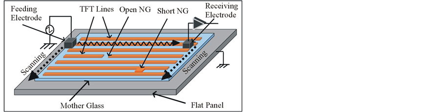
Figure 1. Non-contact FPD inspection system.

Figure 2. A typical pattern of a voltage waveform captured by a noncontact sensor.
2.1. Threshold Based Inspection Method and Its Drawbacks
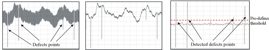
As described above, since the original waveform data captured by a non-contact sensor are full of noises (Figure 3(a)), a moving average filter is applied initially to reduce high frequency random noises (Figure 3(b)). For example if a waveform f of sample size N is given, the resulting waveform g after a moving average filter with a pre-determined subset size p is in the form of:
 (1)
(1)
where fn is the waveform value of f at point n and gn is the waveform value of g at point n. Then the low frequency swinging and baseline fluctuations of the waveform due to the unevenness of the gap between the panel surface and the sensor surface are neutralized by applying a derivative operator (Figure 3(c)). If the waveform after a derivative operator of step length s is h, then h can be expressed as:
 (2)
(2)
The resulting waveform is undergone again a moving average operator to remove remaining spike noises. Finally magnitude values of the waveform are compared with a pre-determined threshold value and the points that exceed the threshold level are considered as defect points (Figure 3(c)).
However, as shown in Figure 3(c), determining a threshold line for discriminating defects points on the waveform is difficult due to the fact that original data are full of noises. Moreover, original captured waveform data are in varying levels of baseline fluctuations. So that in the context of those circumstances the operators always have a severe task of looking data manually and determine proper threshold levels.
2.2. Feed-Forward Neural Network Based Inspection Method and Its Drawbacks
In our previous work [9] [10] , we proposed a feed-forward neural network to classify and detect defect points on waveform data. The structure of the FFN was a 4-layer feed-forward network such that an input layer with two units, two hidden layers with 2 units and 3 units respectively and an output layer with one unit (Figure 4). The inputs to the network were signal to noise ratio (SNR), residual difference, and change of wave length at candidate points on the input waveform. There were 27 weights associated with each input of units, which were optimized by commonly used back propagation training.
 (a) (b) (c)
Figure 3. Detection of defects by thresholding method: (a) Original waveform, (b) After noise suppression, (c) Thresholding on differential waveform.
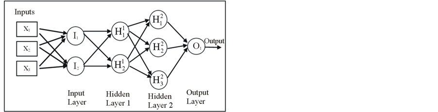
Figure 4. Topology of the feed-forward neural network.
Though this method proved to be much more superior to the existing thresholding method in terms of rate of missed detections and rate of false detections, that method also had its own drawbacks, such as difficulty of picking candidates to the network from noisy data environment and therefore the obvious difficulty of detection. Determining a proper topology of the FNN was also a difficult task which was trial and error based.
3. Proposed Method Using an Evolutionary Optimized Recurrent Neural Network
3.1. Why Recurrent Neural Network?
As described in Section 2.1, the existing criteria of using a threshold for determining defect points on waveforms in non-contact defect inspection method is lacking the appropriateness since the feature variations on and around defect points are largely local features while the deciding threshold is a global value. Also as described in Section 2.2, our previous method based an FNN has its own drawbacks such as difficulties in topology determination process and poor performance in noisy data environment.
After careful observation of the variation of patterns of waveform data from various environments with varying levels of noise levels, we realized that a recurrent neural network would be the best approach to the problem. RNNs are fundamentally different from feed-forward architecture in the sense that they not only operate on an input space but also on an internal state space, a trace of what already has been processed by the network. In other words, an internal feedback can be processed together with external inputs at an RNN. One of the major reasons why an RNN is brought is because it is more resilient on noisy and imperfect inputs
3.2. Input Parameters
Since a neural network can learn from experience, i.e. a neural network can be trained by feeding a known set of data, any feature around an input point on the input waveform that can be considered as influential to the output must be considered as an input to the network. By looking at neighborhood characteristics around defective points on waveforms and comparing with normal area, following three features have been identified as inputs (input vector X) to the network, namely Signal to Noise Ratio (SNR), Residual difference, and Change of wave length. All of these input parameters X(x1, x2, x3) are picked within a pre-determined length of neighborhoods of possible candidate points on the waveform, whereas candidate points are selected by a simple low level threshold such that it may include many false detection but not to miss any defect points.
3.2.1. SNR
If the characteristics within a neighborhood around a defect point on the waveform are observed (Figure 5) it is understood that there is a sharp deviation of magnitude from the normal area. In other words the level of the signal at a particular point shows a considerable deviation against the level of background noise, which means a change of signal to noise ratio (SNR). Therefore SNR is considered as the first component (x1) of the input vector X and is taken as:
 (3)
(3)
where μ is the mean value and σ is the standard deviation of the waveform within the selected neighborhood
3.2.2. Residual Difference
Besides the sharp deviation at the defect point, the neighboring area consisting of a few wave lengths can also be seen deviated towards the same direction as main deviated point (Figure 5). This particular feature of the waveform within the neighborhood is measured as the difference of average upper peak level with the regression line (h1) and the difference of average lower peak level with the regression line (h2). In other words the residual difference of upper and lower peek levels in the neighborhood is taken as the second component (x2) of the input vector X and is taken as:
 (4)
(4)
3.2.3. Change of Wave Length
In the original waveform it shows a considerable change of wave length at a defect point (Figure 6) and is taken

Figure 5. Measurement of SNR and residual difference in a neighborhood of a defect point.

Figure 6. Neighborhood of a defect point on a differential waveform.
as the next input to the network. Though this wave length change appears in the normal waveform, it is easier to measure on the differentiated waveform as seen in Figure 6. So that the rate of change of wave length of a defect point from that of average wave length in the normal area is taken as the third component (x3) of the input vector X and is taken as:
 (5)
(5)
where D is the wave length at the input point and the d is the average wave length at neighborhood (Figure 6).
3.3. Multiobjective Topology Optimization
Choosing an appropriate topology of an RNN to the problem was again a major hurdle as it was even difficult than the previous FNN method by using the trial and error approach. Therefore we decided to use a genetic algorithm based evolutionary optimization approach to determine the topology of the RNN. It is clear that topologies generated by a genetic algorithm may contain many superfluous [13] [14] components such as single nodes or even whole clusters of nodes isolated from the network input. Such units, called passive nodes, do not process the signals applied to the network sensors and produce only constant responses that are caused by the relevant biases. A simplification procedure or a list of constraints can be used to remove passive nodes and links so that the input/output mapping of the network remains unchanged.
By looking at literature [11] [12] [15] -[20] , Delgado et al. [11] proposed a technique for simultaneous training and topology optimization of RNNs using a multiobjective hybrid process based on SPEA2 and NSGA2 [15] . Katagiri et al. [12] introduced some improvements to the Delgado et al. method by introducing an elite preservation strategy, a self-adaptive mutation probability and preservation of local optimal solutions and they have verified their efficiency with benchmark time series data. For this reason, in this paper, we adopt multiobjective evolutionary optimization of training and topology of RNN [12] , for optimizing an appropriate topology of an RNN with the capability of addressing our problem.
The initial topology of the RNN to be optimized will be considered as constructed with one input layer with n units, one hidden layer with m units and a single unit output layer. And a p number of consecutive previous input layers, called past input layers, are copied and kept and are considered as inputs to the hidden layer during each epoch. Similarly a q number of consecutive hidden layers, called feedback layers, are copied and kept and are considered as inputs to the both hidden layer itself and the output layer (Figure 7).
In Figure 7, black arrow lines indicate the inputs to respective layers whereas dashed arrow lines indicate copying of layers to past input layers and feedback layers.
3.4. Optimization Algorithm
The multiobjective optimization algorithm is described in the following 8 steps.
Step 1: Initialize population
Create and initialize a population of chromosomes of size N consisting of each member with an RNN of the topology as in Figure 7. The number of feedback layers, number of past input layers, number of input layer units and the number of middle layer units in all RNNs of chromosomes are set randomly within their respective ranges. A set of training data is also given to the system initially.
Step 2: Evaluate Solutions
Each RNN of chromosomes in the population is trained with back propagation through time (BPTT) algorithm using the given training data set. Since this is the most time consuming step, the patterns of error graphs of each RNN is checked frequently. If the error graph of any RNN goes out of shape from the expected convergence pattern the training process of that particular RNN will be immediately terminated without continuing for the rest of the pre-set number of iterations.
Step 3: Measure fitness
After training all of the RNNs of chromosomes a fitness value is assigned to each chromosome according to a pre-set marking scheme. The marking scheme gives percentage of marks to each chromosome with the following criteria 1) Converged error value 2) Convergence pattern of error graph of its RNN (the better the convergence the higher the marks it earns)
3) Number of neurons in input layer (the fewer the better)
4) Number of neurons in hidden layer (the fewer the better)
5) Number of past input layers (the fewer the better)
6) Number of feedback layers (the fewer the better).
Step 4: Check for the pass mark
If the total fitness level of a particular chromosome exceeds the pass mark (a pre set value, e.g. 90%), the evolution process is terminated.
Step 5: Discard week chromosomes
If the fitness level of a chromosome is lower than a pre-set level (e.g. 20%), that chromosome will be discarded from the populations for not to allow it to mutate or cross over with others
Step 6: Preservation
If the fitness level of a chromosome is bigger than a pre-set level it is considered to be good enough to carry forward to the next generation without mutation or cross over, and the chromosome is flagged and kept.
Step 7: Mutation and Cross Over
Remaining chromosomes are allocated a mutation probability and a cross over probability based on a roulette wheel based selection procedure. Accordingly the chromosomes that mutates will select mutation points randomly and carries on, and similarly the cross over pairs selects their cross over points randomly and performs cross over.
Step 8: Create new chromosomes
Create new chromosomes for discarded chromosomes in step 5 and return to step 2.
4. Experimental Results
4.1. Optimization Results
The evolutionary optimization process, mentioned in section 3.4, was performed with a population of size 40. We observed that the average fitness level of generations was gradually increasing with the evolution as shown in Figure 8. After about 100 generations we found a chromosome with a fitness level over 90%.
The topology of the RNN was optimized to one input layer with 2 units and one hidden layer with 6 units. The number of past input layers were optimized to 3, and the number of previous hidden layers were optimized to 1 (Figure 9). The black arrows indicate the inputs to a certain layer from a certain layer whereas dotted arrows indicate the layer copying.
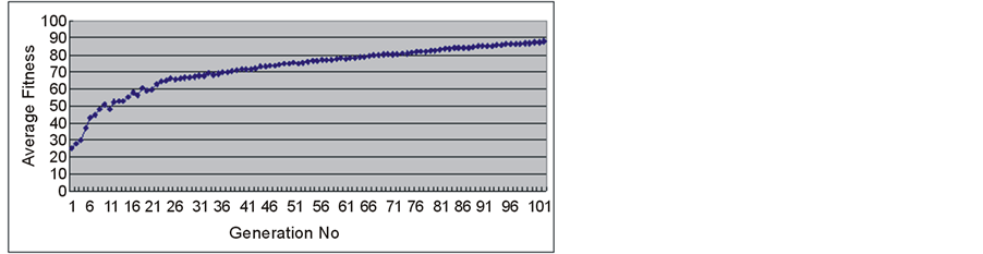
Figure 8. Change of average fitness during evolution.
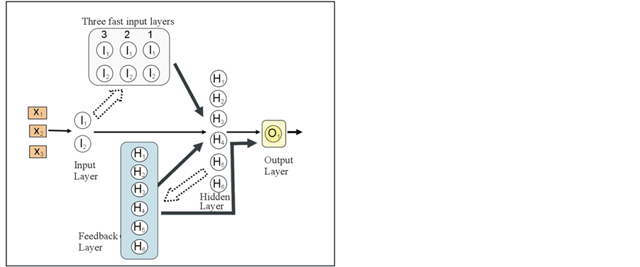
Figure 9. Optimized topology of the RNN.
With this RNN, if the output of the network is  for a given set of inputs X at any given time t, then
  can be explicitly expressed as:
 (6)
(6)
where
 (7)
(7)
where
 (8)
(8)
and
 (9)
(9)
In Equations (6) and (7),  , l = 1,…6, are outputs from the hidden layer and
 , i = 1, 2, are outputs from the input layer at time t.
  and
and  in (6) are weights associated with connections between lth unit of the hidden layer and the output unit and between mth unit of the feedback layer and the output layer respectively. Similarly
 ,
,  and
and  in Equation (7) are the weights associated with the connections between the ith unit in input layer and the lth unit in hidden layer, between the jth unit in feedback layer and the lth unit in hidden layer, and between kth unit in the rth past input layer and the lth unit in the hidden layer respectively.
Also in Equation (8)  is the weight associated with the connection between sth input and the ith unit in the input layer.
4.2. Detection Results
The above optimized RNN was used to detect defect points on waveform data captured by a non-contact sensor over the TFT lines of FPDs. A simple moving average filter was initially applied to smooth the wave data before picking the candidate points to the network. Then the candidate points were selected using a lower threshold value than the threshold value used in [5] -[8] and the three input parameters to the network were picked from those candidate points and entered into the network. Figure 10 shows some detection results on 2 different waveforms captured from 2 different machines in different locations. Both of those voltage waveforms consist of different levels of random noises, external vibrations and baseline fluctuations on them but were able to detect using our method correctly.
The red circles show real defect points while blue dotted lines are candidates and red dotted lines are detected defect points by the RNN among candidates. The left side shows detection in FNN method while the right side shows detection in RNN method in both upper and lower graphs. It shows in both cases that there are some defects points that cannot be detected in FNN method but were possible in RNN method.
We have tested several sets of data and compared results with both thresholding method and our previous FNN method. Table 1 shows a comparison of results using 3 data sets.
5. Conclusions
In this paper, we proposed an alternative method to the problem of non-contact defects detection on flat panel displays using a multiobjective evolutionary optimized recurrent neural network in order to improve the short comings in our previous feed-forward neural network based method as well as in the existing thresholding method. This method does not use any global parameter (pre-determined threshold value) when determining the defect points on voltage waveforms captured by the non-contact sensors. Further, since this method optimizes and determines itself the best topology for the RNN by using a GA based optimization algorithm, it does not require any trial and error based topology selection which was a cumbersome process in the previous FNN based method.

Figure 10. Detection results on two different waveform segments.
To verify the performance of this method, we carried out experiments using 3 types of input data which were captured from different factory environments and different machines. The training data set consisting of 50 defect points and 50 non-defect points was selected from said data and fed into the error back-propagation with time (BPTT) algorithm for optimizing the RNN topology.
By comparing the performance of our method with the existing threshold based method and the FNN method following results were confirmed.
• The existing ratio of missed detection (20% - 30%) in thresholding method and 10% in FNN method was able to decrease below 5%. This is because the evolutionary optimized RNN is more resilient to noise than an FNN.
• The existing ratio of false detection (20% - 30%) in thresholding method and 16% in FNN method was able to decrease below 8%. This is also due to the usage of a trained recurrent neural network for the purpose.
This proves that this method is more feasible and superior than our previous FNN based method and the existing thresholding method for non-contact defect detection. Furthermore by selecting a training data set using every possible scenario, the miss-detection ratio and false detection ratio can be expected near zero.
Acknowledgements
The authors would like to express their gratitude to OHT Incorporation for their generous support and providing their actual data and all the resources and facilities for this research.
NOTES
*Corresponding author.