Population Pharmacokinetic Pharmacodynamic Modeling of Caffeine Using Visual Analogue Scales ()

1. Introduction
Caffeine is a widely used stimulant which acts as a central adenosine receptor antagonist [1] and is frequently ingested to improve energy levels, wakefulness, or even enhance athletic performance [2] . Caffeine is added to beverages (e.g. energy drinks, colas) for the same purpose. Pharmacodynamic effects of caffeine have been evaluated using various assessments such as reflex speed [3] , stylus tapping [4] , or through blood pressure changes [5] . Visual analogue scores (VAS) are widely used in behavioral research and are particularly attractive because of simple administration of the method and the effective use of VAS for evaluation of the caffeine pharmacodynamics has been reported [6] . Determination of an exposure-response relationship between caffeine and its VAS effect may be useful in understanding the quantitative relationships between pharmacokinetics and pharmacodynamics and may assist in clinical trial designs.
Previous publications have used population pharmacokinetic-pharmacodynamic (PK-PD) models to describe other pharmacodynamic effects of caffeine but none have modeled a VAS. Modeling of VAS data is a challenge based not only on its inherent variability (due to subjectivity) but also on the treatment of the data. Depending on the particular VAS used, resulting data may be categorical in which categories are in no particular order, ordinal categorical in which categories have a hierarchical order, or continuous. If the data are either categorical or ordinal categorical, modeling methodology used will estimate the probability of a patient falling into a particular category on the scale. Conclusions from these types of modeling studies will thus report the probability of a patient falling into a particular category based on a treatment or covariate. This methodology is significantly different from the modeling of continuous data which allows estimation of a numerical value corresponding to a specific location on the VAS rather than a probability. Generally, a continuous VAS is standardized to a specific length, such as 100 mm and patient responses are reported as a number which represents the location on the scale at which they indicated their response. For example, on a 100 mm scale, a response reported as 50 would indicate that the individual was at the midpoint of the VAS. In our case, the caffeine analog scale may be treated and modeled on a continuous scale.
Our objective was to develop a population pharmacokinetic and pharmacodynamics model for caffeine plasma concentration data and various pharmacodynamic endpoints assessed by VAS.
2. Methods and Materials
2.1. Study Design
The study was a single center prospective single blinded, cross-over trial and was approved by the Mercer University Institutional Review Board. Twelve healthy subjects, between the ages of 20 and 39 years old (mean 27.2, median 26.5), 11 male, 1 female, each a moderate user of caffeine as defined by an average intake of 2 - 4 cups of coffee daily or the equivalent consumption of caffeine were recruited and given informed consent for the study. Exclusion criteria included a BMI of <19 or >30 kg/m2, concurrent medications with known central nervous system effects including topical formulations and nicotine, concurrent medications with CYP450 interactions, history of drug dependence (excluding nicotine), positive urine drug screen or alcohol test, concurrent chronic or acute illness, hypertension and, for females, pregnant or lactating.
The study consisted of three phases testing three oral formulations of a beverage. Each beverage contained 100mg of caffeine and was provided by The Coca-Cola Company. Other components of each formulation remain proprietary. Prior to the beginning of the study, subjects were randomized to a sequence of beverages to be given at each subsequent visit. Each visit was separated by a minimum of 2 days and a maximum of 8 days.
The subjects were instructed to avoid intake of alcohol for 24 hours, caffeine for 12 hours, and to fast for 8 hours prior to each visit. Subjects arrived at the center prior to breakfast and were given an identical standardized breakfast 1 hour before administration of the study product. Baseline concentrations of plasma caffeine (hereafter referred to as PK) and visual analog scale (VAS) readings (hereafter referred to as PD) were obtained. Following beverage consumption, PK and PD were assessed at 30, 60, 90, 120 and 240 minutes. Additional PK levels were obtained at 360 and 480 minutes.
2.2. Analytical Method
Plasma was separated from blood samples by centrifugation and then frozen until analysis commenced. Plasma samples were prepared for analysis by precipitating proteins using zinc sulfate. Briefly, 100 μL of 2% zinc sulfate (pH 4.5) was added to 200 μL of each plasma sample and then vortexed for 10 minutes at medium speed. The mixture was then centrifuged at 12,000 rcf for 5 minutes [7] . Analysis was conducted using high-performance liquid chromatography (HPLC) (Waters 2690 Separation Module) using a Phenomenex® Kinetex XBC18 column, (4.6 ´ 100 mm, 2.6 um). A gradient elution was utilized with mobile phases consisting of 20 mM sodium acetate and acetonitrile. Flow rate was maintained at 1 ml/min with the temperature held at 45˚C. The retention time of caffeine was 3.3 minutes and detected at 273 nm using a photo-diode array (PDA) detector (Waters 996). Linearity was validated between 200 - 50,000 mcg/L with R2 > 0.999.
2.3. VAS Analysis
The VAS scale (the caffeine analog scale; or Nestle Analog Mood Scale) used in this study has previously been used for determining the effects of caffeine [4] [6] and includes seven mood scales. Each scale was constructed with a horizontal line measuring 100 mm in length with a negative extreme feeling listing on the left and the opposite positive extreme feeling on the right with the midpoint corresponding to a feeling of neither one nor the other. The subject was directed to draw a line perpendicular to the horizontal line of the scale indicating at which point between the two extremes he/she was feeling at that moment in time. The pairs of extremes evaluated were: Lethargic to Vigorous, Muddled to Clear-Headed, Tired to Energetic, Unimaginative to Imaginative, Listless to Full of Go, Ill at Ease to Feeling Fine, and Inefficient to Efficient.
At the completion of the study, a measurement was taken from left to right to assess the subject’s response with a potential maximum movement of 100 mm if the subject ranked their feeling to be the positive extreme for that particular mood.
2.4. Pharmacokinetic and Pharmacodynamic Model Building
The objective was to build a population PK-PD model for VAS data after oral administration of caffeine beverages. Modeling was conducted with NONMEM® (ICON, Ellicott City, Maryland, version 7.2) in conjunction with a g95 (64-bit) compiler using Perl-Speaks NONMEM® (PSN, version 3.5.3) as an interface to run NONMEM®. R (version 2.15.1) and XPOSE4 were used for diagnostic plots. Both simultaneous and sequential PK-PD modeling strategies were attempted. The first order conditional estimation with interaction (FOCEI) method was used throughout the model development.
It was noted that of the 36 visits (3 visits for each of the 12 individuals), approximately 50% of them included a non-zero baseline level of caffeine. To account for baseline levels, an approach was utilized in which a bolus dose of caffeine was input into the depot compartment just prior to the study dose. A rate parameter was estimated as part of the model which defined the pre-dose concentration as described by the exogenous example in the NONMEM® Guides [8] .
Linear one and two compartment models were fit to pharmacokinetic data while linear and Emax models were fit to the pharmacodynamic data. For PD modeling, VAS measurements were treated as continuous variables and a baseline, linear and Emax model were tried:


where E0 is baseline response on VAS, slope is the rate of VAS change based on caffeine concentration, C iscaffeine concentration, Emax is maximal response and EC50 is concentration at half maximal response.
Statistical Model
Between subject variability (BSV) associated with pharmacokinetic and pharmacodynamic parameters was modeled using an exponential model as follows:

where,  is the parameter for the ith subject,
  is the typical value of the parameter in the population, and hi is a BSV with mean 0 and variance ω2. Interoccasion variability (IOV) was tested for some parameters and nested as another level of variability in BSV.
For the pharmacodynamic model, residual variability was attempted as a combined additive and proportional model as follows:

where,  and
and  represent the jth observed and predicted concentration respectively for the ith subject, and ε is the residual random effect. Each ε is assumed to be normally distributed with mean 0 and variance of s2. Reduction of the residual error model to a simpler form was tested during the model development process.
As the pharmacokinetic data was log transformed, a log additive residual error structure was employed as follows:

2.5. Model Selection and Evaluation
Model selection was carried out based on the drop in NONMEM objective function (c2 statistic) as well as assessments of diagnostic plots, evaluation of the clinical relevance of parameter estimates and condition number for signifying model over parameterization. A decrease in the objective function by 3.84 (p < 0.05, 1df) units was considered to be significant. The decision to accept a change in the model was based on a holistic evaluation of the condition of these elements and not on one in particular assessment. Furthermore, successful convergence and covariance steps were required for each model run to be considered for further evaluation.
General goodness of fit plots such as observed caffeine concentrations versus model predicted concentrations, as well as conditional weighted residuals (CWRES) were all utilized in assessing model appropriateness. Distributions of BSV were visualized through histograms to verify that they assumed a normal distribution. Eigenvalues were calculated during the covariance step and used to determine condition number. Each model was evaluated using visual predictive checks [9] (VPCs) using PSN. VPCs were conducted using a sample size of 1000 and the resulting 90% prediction interval (PI) was then compared to the observed values.
A nonparametric bootstrap analysis (n = 2000) was also conducted to estimate the confidence intervals of the parameters without symmetric assumption. Bootstrap runs were excluded if they had a final zero gradient for a parameter estimate.
3. Results
3.1. Pharmacokinetic Model
A one compartment model with first order absorption best described the pharmacokinetics of caffeine and a hypothetical rate of drug infusion was needed to account for the non-zero baseline concentrations (Table 1). Estimation of rate was conducted only on those individuals with a baseline caffeine concentration through the use of an indicator variable. One visit for one individual was excluded from the analysis as their baseline caffeine concentration was over 3000 mcg/L indicating noncompliance with study protocol. Other instances of positive baseline values ranged from 200 - 990 mcg/L which suggest residual caffeine from a short caffeine fasting period. A different rate parameter was estimated for each occasion to avoid the use of interoccasion variability (IOV) as the normality assumption around the rate parameter was not deemed appropriate. Pharmacokinetic parameters of caffeine estimated in the current model are in agreement with previous reports [3] [5] [10] . Based on estimated apparent elimination rate constant (K), population half-life was determined to be approximately 4.3 hours which is in the range consistent with reported values [2] [10] . In the final model, between subject variability (BSV, reported as %CV) was supported on Ka, K and V. Parameter estimates, BSV and bootstrap results are shown in Table 1.
It was found that the addition of IOV on Ka did not improve the model’s overall fit and significantly increased the standard error of the estimate for BSV. Therefore, IOV was not included in the final model.
The final model was not over parameterized as the condition number was approximately 370.
The final model estimated population prediction and the individual subject PK profiles categorized by presence or absence of baseline caffeine concentrations are shown in Figure 2. It should be noted that the addition of the Rate parameter adjusts the population estimate and accounts for the baseline concentration as expected.
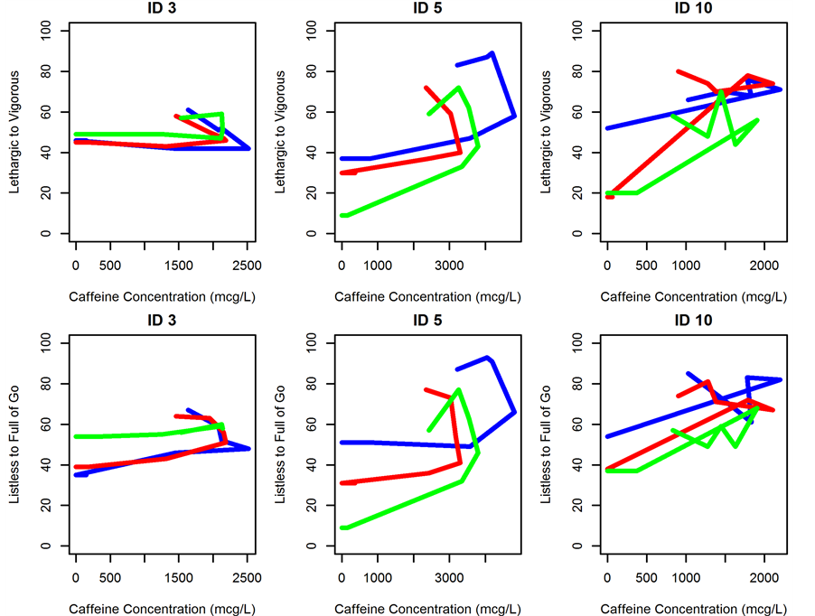
Figure 1. Concentration versus effect plots for individuals 3, 5 and 10 showing counterclockwise hysteresis. Blue line indicates visit 1, red line indicates visit 2 and green line indicates visit 3.
Diagnostic plots of observed versus individual and population predicted concentrations showed reasonable agreement with observed data (Figure 3). Population prediction plots show minor bias for pharmacokinetics around Cmax concentrations but different modeling options attempted did not improve these plots. Population predictions of pharmacodynamic variables were highly variable and thus the plots showed a less coherent distribution of predicted values around the line of unity. Conditional weighted residual plots with time did not show

Figure 2. Concentration versus time grouped by presence or absence of baseline concentration with population prediction. The model was constructed with consideration for baseline caffeine concentration. The left panel shows all visits (indicated by dashed lines and ID numbers) that an individual presented without caffeine concentrations at baseline while the right panel shows all visits with caffeine concentrations at baseline. Solid line represents model estimated population prediction for each group.
major trends indicating no model bias.
VPC plots showed a good agreement between 5th, 95th and median of the simulations and observed data (Figure 4).
3.2. Pharmacodynamic Model
A sequential PK-PD modeling approach was successful. Empirical Bayesian estimates of individual pharmacokinetic parameters were estimated in the PK step and were then imputed to model pharmacodynamics in the second step. Each measure of PD was modeled separately and thus 7 separate models were constructed.
General inspection of the data suggested the presence of delay in effect as Tmax of plasma concentrations preceded the Tmax of pharmacodynamic profile by approximately 1 hour and most caffeine concentration versus VAS effect plots revealed a counterclockwise hysteresis (Figure 1).
The final model that best described the data included an effect compartment where the pharmacodynamic response was modeled with linear slope, baseline effect and was a function of effect compartment concentrations. The final model converged with no errors and a successful covariance step.
Estimation of Ke0, the rate constant which describes the link from the central compartment to the effective compartment, resulted in over paramerized model with condition number >1000 and relative standard error (%RSE) for both Ke0 and slope approached or exceeded 100%. Therefore, as a similar approach to modeling other pharmacodynamic properties of caffeine has been explored by others, we chose to fix Ke0 to 1.73, a value which was reported by a previous publication [2] to allow for a more stable model. A local grid search for Ke0 was conducted by varying the Ke0 value between 1 - 2 (range based on previously published values for Ke0 [3] [5] ) and change in objective function was recorded. PD parameters modeled include E0 (baseline response on VAS) on each occasion and slope (Table 2). BSV was applied to E0 only (reported as %CV, Table 2) and his-

Figure 3. Model evaluation graphs for PK and for all PD variables. For PK, x and y-axis of observations versus predictions are shown in micrograms/liter (mcg/L) while for VAS units are expressed in millimeters (mm).
tograms showed them to conform to a normal distribution (not shown). Concentration in the effect compartment was calculated based on the individual’s PK parameters and the fixed Ke0.
Residual variability was modeled as additive. Resulting parameter estimates, BSV and bootstrap results are shown in Table 2.
Diagnostic plots of observed versus individual and population predicted values (Figure 3) showed good agreement with observed data. Residual plots show no major trends indicating no model bias.
VPC plots show reasonable agreement between prediction intervals and observed data (Figure 5).
An exception exists with regard to the PD variable “Ill at Ease to Feeling Fine”, a variable intended to detect an adverse effect from caffeine rather than determine an effect. Diagnostic plots and other metrics did not show a good fit with any modeling scheme with regard to this variable. A previous publication also reported that this particular measure lacked a relationship to caffeine concentrations which was also found by our model [4] . Therefore, this PD variable was excluded from our analysis.
Condition numbers for all but two of the models were less than 1000. The PD variables “Inefficient to Efficient” and “Muddled to Clear-Headed” were found to have condition numbers of over 1000. However, other diagnostics did not show any other issues with these models.
4. Discussion
Previous publications on caffeine have reported linear pharmacokinetics in both a one compartment [3] [10] and two compartment [5] pharmacokinetic model. In our case, data was found to be best described by a linear, one compartment model with first order absorption and elimination. Because of a short fasting time period for caffeine prior to the study (12 hours), approximately 50% of the visits had non-zero baseline concentrations for caffeine complicating the analysis. In order to account for non-zero baselines, we utilized the bolus dose approach as previously described.

Continued
a. Confidence intervals were calculated through nonparametric bootstrap. Lethargic to Vigorous, n = 2000; Muddled to Clear-Headed, n = 2001; Tired to Energetic, n = 1999; Unimaginative to Imaginative, n = 1994; Listless to Full of Go, n = 1996; Inefficient to Efficient, n = 2000.

Figure 4. Visual predictive check for PK. Dashed lines indicate the boundaries for the 90% prediction interval as determined from the VPC using 1000 samples. The solid line represents the median. Circles indicate observed study data.

Figure 5. Visual predictive check for PD. Dashed lines indicate the boundaries for the 90% prediction interval as determined from the VPC using 1000 samples. The solid line represents the median. Circles indicate observed study data.
Estimated values for pharmacokinetic parameters were similar to those found by others. Three other publications have modeled caffeine PK in a similar manner and found the Ka to be 0.43 [3] , 0.7 [10] and 12 [5] hr−1.The first two values noted are from publications which used a capsule formulation of caffeine while the last value is from a study that tested caffeinated coffee which may contribute to the large difference seen in their model estimated values. Absorption for caffeine occurs rapidly and completely with up to 100% absorption in less than an hour which is reflected by our model [2] . Our estimate of 1.79 hr−1 is reasonable given these previous reports as well as its known quick absorption.
Simultaneous fit of PK and PD was not successful which could be due to high variability in PD. Therefore, a sequential fit was the most appropriate modeling scheme. While there are multiple methods to implement a sequential fit, we chose to use the individual PK parameter (IPP) approach which uses the empirical Bayesian estimates of each participants PK parameters. This method has been shown to give reasonable results when compared to the “gold standard” of simultaneous estimation but is perhaps inferior to the population PK parameter and data (PPP & D) approach [11] . As IPP may add some stability versus the other sequential methods and as we were working with a rich PK sampling and a well-established drug, we felt that IPP was an appropriate methodology. Furthermore, although this method does not allow PD to affect PK, we do not anticipate that VAS data will provide any insight into caffeine PK.
We also employed the use of a theoretical effect compartment which has been done before in modeling caffeine data [3] [5] . The large standard errors estimated for both slope and Ke0 encountered when estimating Ke0, were further evidence of variability in the data. These large standard errors suggest that some individuals may not have any change in their reported VAS score following the caffeine dose which would eliminate both the effective compartment and the slope parameter. However, the majority of subjects for each PD variable did in fact show a response to caffeine data with a rise in VAS scores following dosing. Therefore, to construct a stable model in the face of this variability, we opted to use a previously published value for Ke0 in our PD models. While values published ranged from approximately 1 to 2 hr−1, the value of 1.73 hr−1 was chosen from Shi et al. [5] based on the similarity of our studies in that they both utilized a liquid formulation of caffeine and used a sequential analysis in which the population values were fixed in the PD modeling step. Furthermore, we fixed Ke0 to a range of values between 1 and 2 hr−1 and found little to no benefit for overall model fitness.
Rather than incorporating IOV into our estimation of baseline VAS response (E0) we opted to estimate E0 for each occasion. This approach was utilized as E0 was not expected to be normally distributed which would create a challenge when employing multiple forms of variability which assume normal distribution (BSV and IOV).
A limitation of our study was the lack of a placebo control group. It is likely that a placebo effect would be observed and without this condition, it is not possible to determine what degree of VAS response was due to the placebo effect.
While PK-PD modeling of caffeine has been done before with other pharmacodynamic effects, PK-PD modeling of the caffeine analog scale is reported herein. Modeling VAS data presented a challenge as variability was inevitably high. However, the current model has reasonable predictability of PD and may be useful for future clinical study designs.
5. Conclusion
In conclusion, by employing the exogenous example to handle baseline caffeine concentrations and using a sequential approach coupled with an effect compartment, we were able to link VAS score responsiveness to caffeine concentration in healthy volunteers.