Why Linear Thermodynamics Does Describe Change of Entropy Production in Living Systems? ()

1. Introduction
The main advance in the classic thermodynamics of equilibrium processes in the field of biology is proof that the law of conservation of energy (First law of thermodynamics) is applicable to living systems [1] . However, all attempts to prove that the Second law is true for living systems from the standpoint of classic thermodynamics have failed.
Indeed, the Second law requires that a thermodynamic system evolve to equilibrium in such a way that the total entropy of the system would grow constantly, whereas the rate of its change would decrease. On the other hand, biological processes frequently follow another way, “prohibited” by the Second law. In particular, biological evolution [2] [3] and development of gametes [4] [5] are examples of such a process.
Based on this fact, many scientists have spoken about the fundamental inapplicability of thermodynamics to biological objects [6] -[8] . The researchers who are committed to thermodynamics had to give some explanation to the observed contradiction. In particular, Bauer [9] believed that his law of stable non-equilibrium was not a thermodynamic but rather a purely biological law inapplicable to nonliving systems.
Another direction appeared more beneficial, namely, the formulation of the concept of irreversible processes, which had eventually led to the Prigogine theory [10] -[14] .
Initially, the theory of Prigogine was developed only for systems that are close enough to equilibrium to satisfy the laws of linear form
 (1)
(1)
Ji are thermodynamic flows; Xj are thermodynamic forces; Lij are phenomenological coefficients.
Therefore, this branch of thermodynamics was referred to as “linear thermodynamics” [4] [15] . The main achievement of linear thermodynamics is partition of entropy rate into two components:
 ,
,
 is entropy flow;
  is entropy production.
The entropy flow reflects the mass and energy exchange between a thermodynamic system and its environment and can be both positive and negative. In the latter case, the rate of entropy output exceeds that of entropy input.
Entropy production is connected with various processes within the system and, unlike entropy flow, cannot be negative. According to the Prigogine theory, entropy production is the criterion of evolution of a system. That is why the Second law of thermodynamics for open thermodynamic systems (including living systems) can be put down as .
.
The correlation of entropy production with thermodynamic flows and forces is determined by the dissipative function, which serves as a measured for the energy dissipation,
 . (2)
. (2)
Based on these postulates, Prigogine proved the theorem referred to as the principle of minimum energy dissipation. According to this theorem, any thermodynamic system complying with linear equations Equation (1) evolves in such a way that the energy dissipation determined by Equation (2) constantly decreases and tends to be minimal in a steady state, that is,
 . (3)
. (3)
Inequality Equation (3) is frequently referred to as the criterion of evolution of a thermodynamic system to a steady (or, as a special case, equilibrium) state [4] [16] [17] .
A variant of the Prigogine theory relative to biological objects is the phenomenological theory of ontogenesis, proposed by A. I. Zotin [18] -[22] .
Spread of Prigogine’s theory on the non-equilibrium thermodynamic systems shows that, in general, linear thermodynamics formula Equation (1) (2) and the principle of minimum energy dissipation Equation (3) does not apply to them [13] [16] [17] . Such systems are characterized by excessive energy dissipation. Therefore, they are commonly referred to as “dissipative structures”. Now it became apparent that living systems are dissipative structures [13] . On this basis, some authors believe that the formulas of linear thermodynamics are not applicable for biological processes [23] .
Nevertheless, the linear thermodynamics is capable to describe a large number of biological processes at different levels of organization of living systems: biochemical [24] -[26] , ontogenetic [19] [20] [22] [27] -[29] , environmental [18] [30] , evolutionary [2] [3] .
In this paper, we propose a hypothesis that explains the use of linear equations of thermodynamics processes in biology.
2. Theoretical Propositions
According to modern ideas, there are two fundamentally different types of stable steady states [16] [17] .
First type of the steady states is close to equilibrium. Entropy production in this steady state is positive and determined by the boundary conditions that support entropy production to be constant by external entropy flow. Therefore, it can be considered as a state of relative equilibrium. Special case of the state is absolute equilibrium when the dissipative function is 0. Absolute equilibrium can be achieved only in isolated systems.
Second type is non-equilibrium stable steady states. These steady states should be separated from the state of relative equilibrium by at least one unstable steady state. Increased level of energy dissipation is a characteristic feature of systems in non-equilibrium stable steady state. Therefore, the systems that are near the non-equilibrium steady state were referred to as “dissipative structures”. These include, in particular, living systems.
In this paper, we will consider the specific dissipative function as the main feature, which determines the degree of non-equilibrium systems. We assume the energy equivalent of mass specific rate of oxygen consumption (q) as a measure of specific dissipative function for living systems [4] [18] .
We assume the boundary conditions (environmental conditions) constant throughout the consideration of a thermodynamic system.
Let the rate of the mass specific dissipation function is a continuous function F(q). Let difference between q in relative equilibrium and in absolute equilibrium is negligibly small compared with the current value of q.
Then the function F(q)/q can be expanded in a power series:
 (4)
(4)
In the steady state G(q) = 0. And the roots of the power series Equation (4) correspond to the non-equilibrium steady states.
The dependence G(q) can be represented in the phase plane by curve intersects the abscissa axe at the points of steady states (Figure 1). Stable steady state alternate with unstable. (We don’t consider cases when the curve
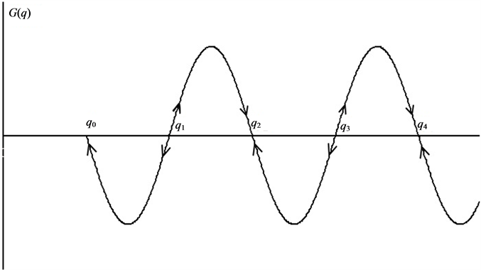
Figure 1. Schematic presentation of the function defined by Equation (4) on the phase plane. Abscissa: mass specific dissipation function. Arrows indicate the directions of evolution of the system. qi are the values of the mass specific dissipation function in the steady states: G(q) = 0. Steady state is stable for even i and unstable for odd i.
only touches zero point. Although system achieves unstable steady state in these points, the general direction of the G(q) does not change). The leftmost point (q0) corresponds to a stable relative equilibrium. Next steady state point (q1) is unstable. If system is not in steady state, it evolves to equilibrium by thermodynamic (left) branch or to the nearest point of stable non-equilibrium steady state by dissipative (right) branch. In the latter case, thermodynamic system forms a dissipative structure.
One expands the function G(q) in a power series with respect to the nearest to the current q stable steady state point qj:

When G(q) is close to the steady state it is mainly determined by the linear member of the series:
 and
and
 (5)
(5)
A = (1 – qi/q0); q0 is value of q at initial time; k = k1.
Equation (5) is equivalent to the corresponding one of linear thermodynamics. The difference consists in the fact that for the nonlinear case k can be a complex number. The real part of the complex number k determines the rate of the system evolution to the steady state. Evolution goes by thermodynamic branch if q0 > qi, and by dissipative branch in the opposite case. The imaginary part corresponds to the oscillation process.
Each stable steady state exists only in a certain period, named characteristic time. If we consider a period much more then characteristic time, the change of entropy production in system cannot be neglected. So, one should include in consideration next stable steady state with more characteristic time. Again increasing the time interval, we obtain the following steady state.
Thus, we can speak about a hierarchy of inserted steady states.
Evolution of the system to the last stable steady state taken into account leads to a change of boundary conditions for all steady states with lesser characteristic time. As a result, for all included steady states qi from Equation (5) is changed. Moreover, if the system is far from the last steady state, changes could be so rapid that one or more inserted steady states could reach the point of bifurcation corresponding to the unstable steady state. When passing this critical point, the whole hierarchy of steady states could be disturbed. This will eventually lead to either build a new hierarchy of steady states, or to the complete collapse of the system as a dissipative structure.
Until now, we did not touch the biological characteristics of living systems. These features are due primarily to ensure that all of the currently existing organisms are the result of a prolonged process of biological evolution, the driving force for which is the survival of the most adapted to the environment species [31] .
In particular, ceteris paribus, those species survive better that are less affected by changes in environmental conditions. The reaction of a living system to change of the environment the weaker the closer it is to the steady state.
Another feature of living systems associated with the survival of organisms, is their ability to alter the level of metabolism spontaneously and, accordingly, the rate of production of entropy. This ability allows organisms to survive adverse environmental conditions. Cases of decreasing in energy metabolism in adverse conditions are widely known. Processes of sporulation, the transition to a hibernation state, falling into a stupor when food or water absent are examples [31] . Those living systems have evolutionary advantages which are closer to the nearest steady state. It is likely that in most cases the deviation of living systems from the steady state is so small that the evolution towards it performs a linear law Equation (1). Then, taking into account Equation (2), the rate of entropy production should change according to the quadratic equation Equation (5).
3. Compliance of the Theoretical Provisions to Experimental Data
Certainly, the use of linear laws to living systems has several limitations. In particular, they are valid only when the changes of boundary conditions can be neglected. That is, parameters of the environment should not change greatly during the data acquisition. One should organize measurements in such a way that the characteristic time of the investigated process would be comparable with the period and the frequency of measurements.
The condition of the organism is also important. At least at the given period it should be only one not yet reached steady state, the evolution to which is the aim of the study. Otherwise, the non-linearity of the system is obvious and application of linear laws becomes impossible.
As an example, we will focus on studies of mass specific rate of oxygen consumption in post-embryonic ontogeny animals. According to some authors, this option, as well as the mass specific rate of heat production, is a measure of the dissipative function in living systems [4] [18] . In these studies the authors usually interested in the change of energy metabolism during aging.
Most authors distinguish only two types of steady states associated with ontogeny: the current steady state with a relatively small characteristic time, and final one, the characteristic time of which is comparable to the lifetime. In order to eliminate the influence of the living system evolution to the current steady state, animals are adapted to the experimental conditions and are led to a state of relative calm. The rate of the oxygen consumption in these animals is called a standard metabolism. To exclude the influence of growth, standard metabolism is usually divided by a unit mass [4] .
Literature dedicated to the study of dependence of the standard metabolism on age is sparse. Nevertheless, all available data confirm the possibility of using the linear law Equation (5) in biology (Figure 2). Values of the coefficients of Equation (5) for different species are presented in Table 1.
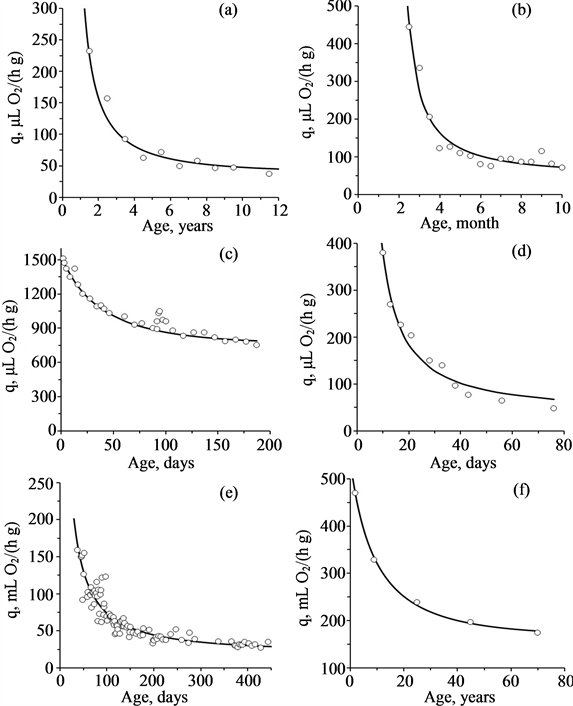
Figure 2. Age-related changes of mass specific rate of oxygen consumption for different species (from [28] ): (a) Mytilus edulis; (b) Lymnaea stagnalis; (c) Acheta domesticus; (d) Drosophila melanogaster; (e) Ambystoma mexicanum; (f) Homo sapiens. Circles are experimental data. Curves are approximation by Equation (5).

Table 1. Coefficients of Equation (5) for post-embryonic development of different species.
Notes: values qi are given at 20˚C for poikilothermes and in the thermoneutral zone for homoiotherms. Calculations of qi for bivalves are based on the weight of soft tissues (without shell).
Equation (5) contains only three easily interpretable constants: qi is the value of q in the steady state; k is the coefficient associated with the characteristic time of the process; A is the constant of initial conditions.
Simplicity of the equation allows its use in biology to determine species’ longevity, to compare the level of standard metabolism in different individuals, populations, and species [28] [32] -[35] , etc.
Of course, the formula Equation (5) describes only the basic trend of evolution to only one steady state. For a complete description, we should also take into account the evolution of the system to all the unreached steady states and wave processes that accompany each steady state. We will consider these problems later.
4. Conclusions
Thus, dissipative structures, which include living systems, have several steady states with different characteristic time of their achievement. Change of one of the stationary states leads to change in boundary conditions for all stationary states with lesser characteristic time. The greater the change, the greater the probability that the bifurcation point will be achieved by deviation from at least one stationary state. If it happens, restructuring of the entire hierarchy of stationary states take place or the system will cease to exist as a dissipative structure. The more system deviates from the steady state, the faster boundary conditions for “embedded” steady states changes, and the greater the probability of destruction of the system is.
One usually calls the entire hierarchy steady states by the term “homeostasis”. Existing living systems are the result of long-term biological evolution. It is clear that an evolutionary advantage given to those organisms that ceteris paribus are able to maintain a state of homeostasis for a longer time. Therefore, biological evolution should lead to the formation of systems with minimal possible deviation from the stationary states. The proximity of living systems to any of the steady states leads to opportunity of linear approximation for the description of system evolution to this steady state. I believe that this explains the possibility of linear thermodynamics to describe the processes in living systems, including change of entropy production.
Acknowledgements
This work was supported by RFFI (grant number 12-04-00397-a), and the Presidium of the Russian Academy of Sciences under the programs “Wildlife: Current Status and Problems of Development”.