Multilevel B-Spline Repulsive Energy in Nanomodeling of Graphenes ()
1. Introduction
Nanotechnology is a very important field which has emerged in the last decades and developed very quickly in several directions. It has important applications in various disciplines including aircraft, automobile, electronic and medical engineerings. Nanomaterials admit several important properties which can be exploited in applications. For instance, electric conductivity of nanomaterials is applied in electronic components so that the materials conduct electricity more efficiently than diamonds. Thermal resistivity of nanomaterials can be used to reduce or accelerate heat conduction. It also has a good thermic property so that materials can be designed to resist heat at a very high intensity. Graphene has obtained a significant attention from scientists in the last decades for several reasons. Its material property can be controlled for that it can become a stronger material than steel. The objective in this paper is to use an accurate and efficient fitting of the repulsive energy instead of using a standard parametrization. Many approaches have been proposed to represent empirical estimation of repulsive terms. Before presenting our method, let us briefly survey some traditional repulsive methods. Molecular dynamics employing the Lennard-Jones potential have been well understood so far. It is based upon the well-known potential
 (1)
(1)
which is decomposed into attractive and repulsive components. Since it is only expressed in terms of the inter-atomic distances, it is easy to handle. Due to the simple expression of the potential, it can be differentiated easily and it is not computationally expensive to evaluate. Another important parameterization is the Harrison parametrization:
 (2)
(2)
The screened Harrison parametrization is an improvement of the former one as provided by
 (3)
(3)
where  controls the range of the interaction and
  is some parameters obtained by experiments or a fitting process. Sawada parameterization uses the expression
 (4)
(4)
The most currently used parametrization is the GSP parameterization (Goodwin-Skinner-Pettifor) which is expressed as
 (5)
(5)
where ,
,  and
and  are fitting parameters. Several other methods have been also suggested to achieve some desired properties. Some approaches use certain combinations of known ones.
Our motivation is to generate a system which is both accurate and fairly inexpensive to evaluate. We are interested in graphenes and its properties including energy, force and elastic stress. Geometrically, graphenes admit a honeycomb pattern in form of repeated organized hexagons as illustrated in Figure 1(a). They are controlled by the chirality which is a couple of integers  so that
 . In the case
 , one has an armchair graphene while
  corresponds to the case of a zigzag graphene as in Figure 1(b). Suppose
  designates the carbon bond length of the graphene. Define
  and
and  the directive vectors of the honeycomb describing a 2D-lattice so that
  and
and . The chirality indices
  produce the chirality vector
 . For the generation of the unit cell, one needs a translational vector
  perpendicular to the chiral vector
 . Let
. Let  designate the greatest common divisor of
  and
and . Define
  if
if  while
while  otherwise. The translational vector is expressed by
 . In the following sections, scaling a graphene amounts to enlarging the unit cells by scaling its primitive vectors. The coordinates of the centers of carbon atoms in the unit cell provided as fractional coordinates within
  remain unchanged. We are interested in the property of the graphenes as they are confined or stretched as illustrated in Figure 1(c) where we consider a graphene of chirality
 . For significantly confined graphenes, the repulsive energy is very large. For extremely stretched ones, the repulsive energy vanishes so that the energies are the sum of the energies of all constituting atoms.
2. Quantum Repulsive Representation
We consider the Born-Oppenheimer or adiabatic approximation assumption stating that the mass and the volume of the atoms are very large in comparison to those of the electrons. The atoms move comparatively slower than the electrons. Thus, we treat the time-independent Hamiltonian operator with respect to the a set of nuclei  which are supposed to be stationary:
 (6)
(6)
where the coordinates of the  -th electron are denoted by
  and
and . The above formula describes the kinetic energy along with the nuclear-electron interaction and the inter-electron interaction. Several simplifications of the stationary Hamilton operators have already been proposed. Our proposed potential energy uses two of such simplifications which we survey below.
For the DFT(Density Functional Theory), one solves one equation for each electron. The Kohn-Sham formalism [1] consists in replacing the complicated single problem into several simpler ones. For each 
 (7)
(7)
where  is the effective potential energy which depends implicitly on the total electron density
  such that
 . The problem is then reduced from dimensions
  to
to  sets of smaller problems of dimension
 . The influence of one electron with respect to the other electron is measured by the total electron density. These approaches enable the treatment of Hamiltonian problem even for an electronic structure having a large number of particles on a single desktop. The eigenvalue problem in (7) is nonlinear because its variational [2] [3] operator
  depends on
which in turn depends on . It is solved by using a sequence of the linear eigenvalue problems SCF (Self Consistent Field). The effective potential is constituted of the Hartree potential
 , the exchange correlation potential
  and the external electrostatic field such as

in which the Hartree potential is the inverse of the Poisson operator such as . For its evaluation, either a Poisson problem is solved or one convolves with the Green fundamental solution such as
 . The main feature of DFT is that one has to approximate the potential by using some correction terms known as exchange-correlation potential [4] [5] . That is usually done by LDA (Local Density Approximation) or GGA (Generalized Gradient Approximation). Analytic expressions of the correlation energy are only known in a few special cases which mainly consist of the high and low density limits. The external electrostatic field potential
  is provided by the kernel
 . The above exchange-correlation potential is related to the exchange-correlation energy by
  where one expresses
  as the exchange and the correlation parts. In term of the exchange-correlation energy density
  one has
 (8)
(8)
where . For the local density approximation (LDA), the exchange energy density is expressed as
 so that
 . Analytic values of the correlation energy density are only known for some extreme cases. For the high density limit, the exchange correlation energy density is approximated by
  when the Weigner-Seitz radius
  is very small. For the low density limit where
  is very large, one has
 . For other values of
 , some interpolation of those extreme values is considered. For example, by using the VWN-approximation (Vosko, Wilk, Nusair) as in [6] , one has

where  while each one of
 ,
,  and
and  is of the form

in which ,
,  and
and . The constants
 ,
,  ,
,  ,
,  are fitting parameters which are different for
 ,
,  and
and . Once the solutions
  to (7) become known for all
 , the Khon-Sham approach uses the approximation to
  of (6) by

The main improvement from LDA to GGA is that the exchange-correlation energy does not depend only on the total electron density but also on its gradient such as .
.
As a second simplification, we survey the semi-empirical (SE) method using Hueckle method. Consider the spherical coordinates  such that
 . The spherical harmonics
  is provided by

and

The atomic orbitals sharp (s), principal (p), diffuse (d) and fundamental (f) correspond to linear combinations of  for
for  respectively. The basis functions centered at the origin are [7] defined by
  where the radial function
  is given by

The parameters  are specified for each atomic orbital. Since one has a set of atomic centers
 , one associates to each center
  several atomic orbitals and indices
 . The overlap matrix entry for the centers
  and
and  is designated by
 . For the on-site case where the bases are centered at the same atom
 , the SE Hückle method provides
 . That is, the on-site bases are mutually orthonormal. For the nondiagonal values or off-site cases centered at two different atoms
  and
and , the entries are computed by a Slater-Koster table lookup where the values are functions of the interatomic coordinates
 . In fact, the overlap matrix entries can be expanded as
where one uses the inter-atomic distance . Computing the integrals by quadrature is too expensive.
One stores the expansion coefficients . The value of
  are stored in Slater-Koster table. It does not depend on the coordinates of
  and
and  but only on the inter-distance (see [7] for similar discussion). For the Hamiltonian of the SE Hückle, the on-site situation with respect to the center
  is
is

where  is approximately the eigenenergy for index
 . The off-site term is

The value of  is the solution to
 . This partial differential equation needs to be solved for every evaluation of the Hartree term
 . In the Atomistix Toolkit package [7] , that is solved by a fast multigrid solver. The coefficient
  is a dielectric coefficient [8] and
  is a certain induced electron density.
As a matter of fact, the SE empirical method is much more efficient than the DFT method in term of computational speed. But the DFT computation produces much more accurate results. As a consequence, one searches a certain correction term for the SE method in such a way that the resulting method keeps the efficiency of the SE method while approximating the quality of the DFT approach. The ultimate objective is thus to find a repulsive term to add to the SE energy as described below. We want to generate a repulsive term which conserves most of the properties from the DFT computation. For a configuration , we intend to conserve the energy
  such that
 . In addition, we are also interested in approximating the forces. For each atom
 , the corresponding force is
such that . In addition, we focus also on the elastic property of the graphenes [9] . In general, this property determines the rigidity of a graphene when a traction is applied on it. The strain tensor which is
 (9)
(9)
is represented in the longitudinal, transversal and normal components. The stress  is also represented in a similar tensor way. The strain is related to the displacement
  having components
  by
by . The correlation between the strain
 , stress
  and displacements
  is governed by some elasticity equation [9] . Practically, the stress contains implicitly some property of the second derivatives of the energy for the reason that it is the derivative of the energy with respect to strains which are functions of the gradients of the displacements
 .
.
For a set  of graphene configurations, the ideal objective functional for the nonlinear optimization is
 (10)
(10)
In the above expression,  designates a scaling of a configuration
  by a factor of
 . In addition,
  ,
,  ,
,  are sets of scaling factors with respect to the reference configuration
  for the energy, force and stress respectively. Now, we show the construction of
  and
and  where considers the interval
  which prescribes the range of interest. That interval contains the optimal factor
 obtained from a geometry optimization. The construction is performed in several steps as depicted in Figure 2. As a first step, one refines the interval
  uniformly. Afterwards, one refines gradually in the vicinity of the optimal scaling factor
  of the configuration
 . The principal objective for that construction is to accumulate many points in the neighborhood of the optimum
 . The determination of the stress is computationally more intensive compared to the computation of the energies. That situation holds even for the case of semi-empirical Hueckle method. The computation of stress for the DFT case is even more intensive but it needs only be done once and stored during the whole optimization. As a consequence, one needs only to handle elastic properties at a few positions in the course of the optimization computation. Otherwise, the whole optimization execution would be too slow since the evaluation of the objective functional would be very intensive. For example, the stress is only applied in the neighborhood of the minimal energy in our computation. Generally,
  is smaller in size than
  and
and . Not all the range of the scaling factor
  is of the same importance. The vicinity of the optimal scaling factor
  is more valuable because the equilibrium takes place there. As a consequence, one introduces some positive weights to the scaling factors. For our implementation, we used some Gaussian functions centered at the optimal value added by some minimal shift
  such as
 (11)
(11)
The purpose of  is to prevent the value of
  from being practically zero when
  is far from
 . In our case, we have taken the parameter values to be
  and
and . Since the objective function (10) is very intensive to evaluate, we use in practice its simplification where the forces are provided by finite difference of the energy. Now we would like to describe the parameters with respect to which the nonlinear optimization is performed. The semi-empirical energy with zero repulsive term
  behaves as a pure attractive energy. That is, in order to obtain an energy comparable to the DFT energy, one appends a
repulsive energy in form of sums of pairwise potential terms such as

That is, the function  acts pairwise on the carbon atoms with nuclei coordinates
  and
and  such that
 . In other words, the whole process amounts to replacing the repulsive term of the SE energy by an optimal potential energy
 . We search for the optimal pair potential function in the form
 (12)
(12)
in which  designates B-spline basis functions such that we obtain an energy that behaves very similarly to the DFT in term of energy, force and stress.
In the expression (12), the function  captures the general behavior of the pair potential function
 . The role of the B-spline
  is to correct the small imperfection produced by the principal function
 . Some cut-off radius
  is used so that the pair potential function
  vanishes beyond that value. In our situation, a cut-off radius of about
  Å suffices completely. In order to obtain zero value and derivative
 , we insert a short transition function next to the cut-off radius
 . One extends
  next to the cut-off radius
  by a polynomial so that one obtains a smooth transition toward zero.
Since the unknown pair potential function is partly expressed in B-spline basis as in (12), we recall briefly some important properties of a B-spline setting. It is in fact a very flexible way of representing piecewise polynomials on any interval of definition . Consider two integers
  such that
 . Suppose the interval
  is subdivided by the knot sequence
  such that
  for
for  while
while  and
and . One defines the B-spline basis functions for
  as
as

where one employs the divided difference  in which the truncated power functions
  are given by

We only focus on B-splines which are internally uniform: except for the boundary multiple knots, all knot entries  are uniformly spaced. The integer
  controls the smoothness of the B-spline for which the resulting function admits an overall smoothness of
  so that the case
  corresponds to discontinuous piecewise constant functions. The integer
  controls the number of B-spline functions. In Figure 3(a), we see some illustration of B-spline bases on an internally uniform knot sequence. Figure 3(b) displays an instance of a B-spline curve defined on
 . In Figure 3(c), the knot sequence has been refined uniformly by increasing
  to
to  while keeping
 . That is achieved by introducing a new knot entry between every two knots of the B-spline in the former Figure 3(b). For our application, we insert several knots at once so that the new knot sequence is again internally uniform. A new knot entry is inserted between two consecutive old ones. The evaluation of B-spline functions is not calculated by using the above definition but rather by means of the de-Boor algorithm. Since the knot sequence is internally uniform, we use the notation
  instead of
  in (12). We will describe next the procedure of inserting new knots into existing ones. That is important when one needs to increase the degree of freedom in the pair potential function in (12). The principal objective is to efficiently express a function defined on the coarse knot sequence in term of B-splines on a fine one. Consider two knot sequences
  and
and  such that
 . For both knot sequences, the smoothness index
  is conserved intact. The following discrete B-splines enable the expression of a coarse basis
  as a linear combination of the fine basis
 . Choose
  and define
 (a)
(a) (b)
(b)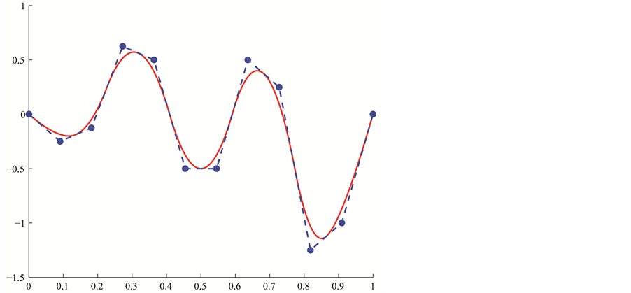 (c)
(c)
Figure 3. (a) B-spline bases; (b) Original B-spline; (c) a finer B-spline which has the same parametrization as the original B-spline.
where . One has

where . The discrete B-splines
  are evaluated by using the recurrence

in which

In our simulation, we took  which corresponds to continuously differentiable pair potentials. In Figure 4, we observe some illustration of such knot insertions. Not only the two B-spline functions admit the same image but their parametrizations from their interval of definition
  are completely identical.
The whole process of the determination of the repulsive energy is performed in increasing levels as follows. First, one determines the optimal value for  without the B-spline part in (12) by using a global optimizer. Then, one fixes the resulting optimal values of
  during the subsequent computation. Second, one searches the optimal B-spline
  where
where  by starting a local optimization with the initial guess
 . Now, one repeats the following steps iteratively. Inject the optimal value
into  by using the above knot insertion technique where
  is increased into
 . Apply then a local optimization with respect to
  by using,
  as initial guess.
3. Computer Implementation
In this section, we report on some practical results of the formerly proposed method. The implementation of the method was realized by combining ATK, NLOPT and python. The ATK (Atomistix ToolKit) has some GUI extension well known as VNL (Virtual NanoLab). We use NLOPT for the diverse nonlinear optimization operations [10] in which both global and local optimizers are involved. A global optimizer searches for the best parameters among all possibilities while a local one searches only inside a local neighborhood of a certain provided starting initial guess. For the global optimizer, we use the NLOPT option GN-CRS2-LM standing for Controlled Random Search with Local Mutation. The local optimizers are performed by using BOBYQA algorithm which is an efficient gradient-free method available in NLOPT. In order to facilitate the combinations of options, we implemented several python classes. The class for the reference configurations organizes the graphene structures to be used together with their respective optimization weights. There is also a class for the optimization parameters specifying the property such as orders and levels of B-splines as well as the abortion criterion. It controls the contribution of the energy, force and stress  in the optimization functional (10). The construction of the sets
  as well as the interval for the range of interest has been equally supported by some python classes. In order to save computations, one needs to precompute and store the data for the DFT as well as the semi-empirical with zero pair potential.
As a first test, we consider multiple computations for different configurations of graphenes. The configuration  is based upon the first index
  of the chirality parameters
  where
where  is allowed to vary. That is, each configuration
  is composed of all graphenes admitting chirality
  such that
 . In Figure 4(a), we observe some comparisons for graphenes in
  where
where . Most values align on the diagonal which implies the agreement between the outcomes provided by the DFT and the SE methods. Similar tests for graphenes where
  and
and  are depicted respectively in Figure 4(b), Figure 4(c). The resulting SE energies do not exactly provide the same results as the DFT but the current SE energies should be more reliable in comparison to the empirical potential in (1)-(5) which contain very few parameters. In addition, the speed of computation is much faster for the currently presented SE than the one for DFT. In fact, the execution time of
the SE in comparison to DFT has a speed of factor  or more. Due to that acceleration gain, the method is in many aspects good to attain efficiency. If the accuracy is not satisfactory, then one has to use the direct DFT with the cost of much more computing time.
As a further test, we investigate the decrease of the objective function with regard to the B-spline levels. We consider again the three configurations  above for
 . The results of such tests are displayed in Table 1 where the initial line describes the SE with zero pair potential (PP). The next one is the SE with exponential pair potential
  without B-splines. The following ones are the pair potentials with more and more B-splines as in (12). The error barely drops down after level
  for all graphene configurations
 . In fact, the minimal value of the function in (10) is not always zero. As a consequence, one cannot expect an arbitrarily accurate approximation. As a next test, we consider the complex band structures for using the DFT and SE computations whose results are respectively displayed in Figure 5(a), Figure 5(b) for the graphene with chirality
 . The plots depict band lines which are not shown as continuous curves but as sets of sampling points. The points which are purely real and explicitly complex are depicted in red and green respectively. In order to provide more validation for the efficiency of the proposed method, some comparison of the elastic properties was performed when computed by means of the DFT and SE methods. In Figure 6, we observe the elastic properties corresponding to the two methods. In general, the stress tensor
  is presented in three directions similar to (9). Nevertheless, we omit the normal components of the stress tensor
  in this particular
 (a)
(a) (b)
(b)
Figure 5. Complex band structures. The purely real values are shown differently for : (a) Using DFT; (b) Semiempirical.

Table 1. Errors at each B-spline level.
case of the graphene configurations which are planar. In addition, the stress components  and
and  are practically zero for both the DFT and SE computations. As a result, it remains to consider the longitudinal component
  and the transversal component
 . That is, we need only to compare between
  and
and  as well as
  and
and . We concentrate only on
  because the other configurations produce similar results. The cases of graphenes admitting chiralities
  and
and  are respectively shown in Figure 6(a), Figure 6(b) where one observes the alignments of DFT and SE elasticities. The two results for
  and
and  are almost similar except that
  corresponds to
 . Geometrically, the transversal direction of the chirality
  corresponds to the longitudinal direction of the chirality
 .
.
4. Conclusion
A method was presented to determine the optimal pair potential for the repulsive quantum energy. We concentrated on configurations which are constituted of carbon graphenes. The method was based upon hierarchical B-splines layered on different levels. The principal objective function consists of terms involving not only energies but also forces and elastic stresses. Several computer results validate the reliability of the newly proposed method as compared to outcomes from Density Functional Theory.