Decompositions of Symmetry Using Generalized Linear Diagonals-Parameter Symmetry Model and Orthogonality of Test Statistic for Square Contingency Tables ()
1. Introduction
Consider an  square contingency table with the same row and column classifications. Let
  denote the probability that an observation will fall in the ith row and jth column of the table
  Bowker [1] considered the symmetry (S) model defined by
This model describes the structure of symmetry with respect to the cell probabilities  As a model which indicates the structure of asymmetry for
  Agresti [2] considered the linear diagonals-parameter symmetry (LDPS) model defined by

A special case of this model obtained by putting  is the S model. Yamamoto and Tomizawa [3] considered the generalized linear diagonals-parameter symmetry (LDPS(K)) model as follows; for a fixed
Especially the LDPS(0) model is equivalent to the LDPS model.
Let for 
 and
and 
The S model may be expressed as

Thus the S model also has the structure of symmetry with respect to the cumulative probabilities 
 Miyamoto et al. [4] considered the cumulative linear diagonals-parameter symmetry (CLDPS) model defined by

which indicates a structure of asymmetry for 
 The CLDPS model is different from the LDPS model. Yamamoto and Tomizawa [3] considered the generalized cumulative linear diagonals-parameter symmetry (CLDPS(K)) model as follows; for a fixed

Especially the CLDPS(0) model is equivalent to the CLDPS model.
Let  and
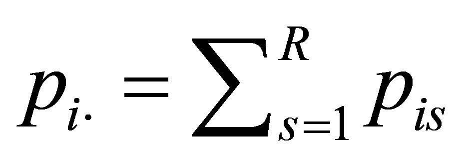
and  denote the row and column variables, respectively. We consider the mean equality (ME) model as
where  and
and 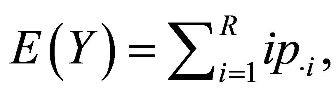
 and
and 
Yamamoto et al. [5] gave Theorem 1. The S model holds if and only if both the LDPS and ME models hold.
Yamamoto and Tomizawa [6] gave Theorem 2. The S model holds if and only if both the CLDPS and ME models hold.
The present paper gives several decompositions of the S model using the LDPS(K) and CLDPS(K) models. It also proposes the mean nonequality model, and gives the orthogonal decomposition for testing goodness-of-fit of the S model. An example is given.
2. Decompositions of Symmetry Model
We shall give five kinds of decompositions of the S model using the LDPS(K) and CLDPS(K) models.
Theorem 3. For a fixed  the S model holds if and only if both the LDPS(K) and ME models hold.
Proof. If the S model holds, then both the LDPS(K) and ME models hold. Conversely, assuming that the LDPS(K) and ME models hold and then we shall show that the S model holds. The ME model may be expressed as

From the LDPS(K) model, we see

Therefore we obtain . Namely the S model holds. The proof is completed.
Theorem 4. For a fixed  the S model holds if and only if both the CLDPS(K) and ME models hold.
Considering the global symmetry (GS) model as

namely

we obtain Theorem 5. For a fixed  the S model holds if and only if both the LDPS(K) and GS models hold.
We shall omit the proofs of Theorems 4 and 5 because these are obtained in a similar manner to the proof of Theorem 3.
For a fixed  consider the mean nonequality (MNE(K)) model as follows:
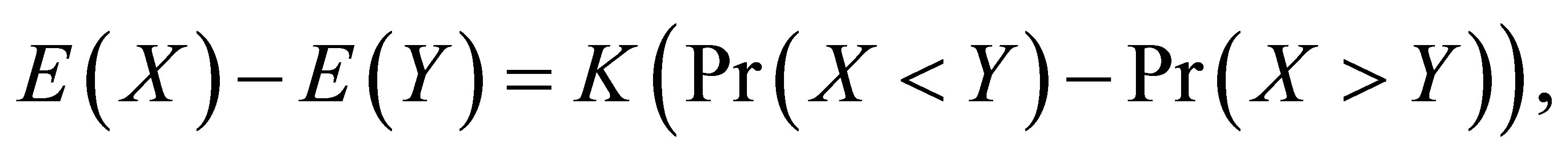
which is

This model indicates that the difference between the means of  and
and  is
is  times higher than the difference between the global symmetric probabilities. When
  the MNE(0) model is identical to the ME model. We obtain Theorem 6. For a fixed
  the S model holds if and only if both the LDPS(K) and MNE(K) models hold.
Theorem 7. For a fixed  and for a fixed
  the S model holds if and only if both the LDPS(K) and MNE(L) models hold.
We shall omit the proofs of Theorems 6 and 7 because there are obtained in a similar manner to the proof of Theorem 3. Note that: 1) Theorem 6 is an extension of Theorem 1 because when  Theorem 6 is identical to Theorem 1; 2) Theorem 7 is an extension of Theorem 3 because when
  Theorem 7 is identical to Theorem 3; and 3) Theorem 7 is an extension of Theorem 6 because when
  Theorem 7 is identical to Theorem 6.
3. Test Statistic and Orthogonality
Let  denote the observed frequency in the ith row and jth column of the
  table with
  and let
  denote the corresponding expected frequency. Assume that
  has a multinomial distribution. The maximum likelihood estimates of expected frequencies
  under each model could be obtained, for example, using the Newton-Raphson method to the log-likelihood equations. Each model (say, model
 ) can be tested for goodness-of-fit by the likelihood ratio chi-squared statistic
  with the corresponding degrees of freedom, defined by

where  is the maximum likelihood estimate of
  under the model. The number of degrees of freedom for the S model is
  and that for each of the LDPS(K) and CLDPS(K) models is
  (being one less than that for the S model). That for each of ME, GS, and MNE(K) models is 1. Note that the number of degrees of freedom for the S model is equal to the sum of those for the decomposed models.
Lang and Agresti [7] and Lang [8] considered the simultaneous modeling of a model for the joint distribution and a model for the marginal distribution. Aitchison [9] discussed the asymptotic separability, which is equivalent to the orthogonality in Read [10] and the independence in Darroch and Silvey [11], of the test statistic for goodness-of-fit of two models (also see Tomizawa and Tahata [12], Tahata et al. [13], and Tahata and Tomizawa [14]). On the orthogonality of test statistic for models in Theorem 6, we obtain.
Theorem 8. For a fixed  test statistic
  is asymptotically equivalent to the sum of
  and
and 
Proof. The LDPS(K) model may be expressed as
 (1)
(1)
where  Let
Let


where “t” denotes the transpose, and

is the  vector. The LDPS(K) model is expressed as

where  is the
  matrix with
  and
and  is the
  vector with

where

and  is
is  matrix of 0 or 1 elements determined from (1). The matrix
  is full column rank which is
  In a similar manner to Haber [15], Lang and Agresti [7], and Tahata and Tomizawa [16], we denote the linear space spanned by columns of the matrix
  by
by  with the dimension
  Note that
  where
where  is the
  vector of 1 elements, and thus
  Let
Let  be an
be an  where
where  full column rank matrix such that the linear space
  is the orthogonal component of the space
  Thus,
Thus,  where
where  is the
  zero matrix. Therefore, the LDPS(K) model is expressed as

where  is the
  zero matrix, and

The MNE(K) model may be expressed as

where 
Note that  From Theorem 6, the S model may be expressed as

where 

Note that  are the numbers of degrees of freedom for testing goodness-of-fit of the LDPS(K), MNE(K) and S models, respectively.
Let  denote the
  matrix of partial derivatives of
  with respect to
  i.e.,
i.e.,  Let
Let  where
where  denotes a diagonal matrix with ith component of
  as ith diagonal component. We see that

because  and that
Thus we obtain

Therefore we obtain  where
where

From the asymptotic equivalence of the Wald statistic and the likelihood ratio statistic (Rao [17], Darroch and Silvey [11], Aitchison [9]), we obtain Theorem 8. The proof is completed.
4. Analysis of Data
Table 1 taken directly from Agresti [18, p. 232] summarizes responses to the questions “How successful is the government in (1) providing health care for the sick? (2) Protecting the environment?”.
Table 2 gives the values of the likelihood ratio test statistic  for models applied to these data. The S model does not fit these data so well. Also, each of the ME (i.e., MNE(0)), MNE(K)
  and the GS models does not fit these data so well. However each of the LDPS(K) models
  and the CLDPS(K) models
  fit these data very well. Using Theorems 3 through 7 (including Theorems 1 and 2), we shall consider the reason why the S model fits these data poorly. For the structure of cell probabilities
  we see from Theorems 3, 5, 6 and 7 that the poor fit of the S model is caused by the influence of the lack of structure of the ME model (the GS model or the MNE(K) model
 ) rather than the LDPS(K) model
  For the structure of cumulative probabilities
 we see from Theorem 4 that the poor fit of the S model is caused by the influence of the lack of structure of the ME model rather than the CLDPS(K) model