Euler-Lagrange Elasticity: Differential Equations for Elasticity without Stress or Strain ()
1. Introduction
Euler, Lagrange, and Poisson all described the deformation of materials in terms of positions of points and forces within the body. Cauchy introduced the concepts of stress and strain, which are now the standard for elasticity equations (An accessible early history is found in Ref [1] with pointers to the source documents). In this paper, I will return to the earlier use of points and forces to describe elasticity. Surprisingly, only a few basic assumptions are required.
2. The Differential Equations
Using the notation of Spencer [2], the points within the body before deformation are described as Xi = (X1, X2, X3), with  corresponding to the initial x, y, and z coordinates of each point, respectively. The corresponding points within the body after deformation are described as
 . The position of each point after deformation is a function of the original location of that point, i.e.
 , x2 = f2(X1, X2, X3), and
 .
.
When an elastic material is deformed, work is done on the material and energy is stored in the material. As the material is returned to its original shape, the energy returns to its original value. Thus the energy depends only upon the final position of the points within the body. Experts in elasticity theory call this hyperelasticity. Hyperelasticity will be assumed for the remainder of this paper.
The differential equations are derived by assuming the energy per unit volume of the material is a function of the final point locations,  , and the relative displacements of near-by points,
 . The total energy of the body is then
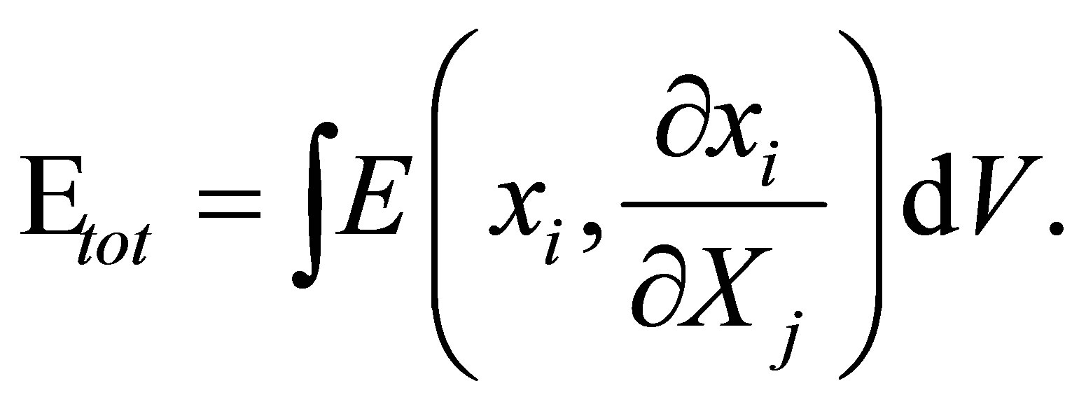 (1)
(1)
It is also assumed that when the body is moved or deformed, the internal points within the body move so as to minimize the total energy. That is
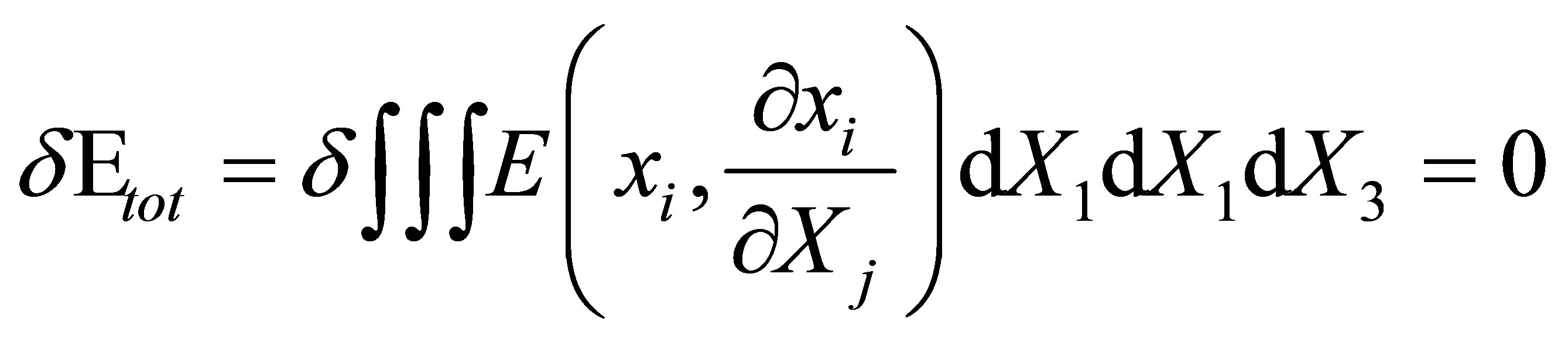 (2)
(2)
for i = 1, 2, 3 and j = 1, 2, 3 and where the integral is taken over the entire body.
Minimizing this energy function Equation (2) results in the following three Euler-Lagrange equations,
 (3)
(3)
These are the differential equations of elasticity. All that remains is to appropriately describe the energy function E and the boundary conditions.
2.1. Energy
To describe the energy per unit volume E, divide the energy into two parts.  which defines the energy associated with body forces and
  which defines the energy associated with the deformation of the body.
  is typically only a function of the positions of the points within the body. (e.g., the energy per unit volume associated with a gravitational force would be just
 , with the
  axis vertical.)
  is typically a function only of the relative positions of the body, i.e. a function only of
 . The total energy associated with the body is then the sum of the contributions from these different energies,
 (4)
(4)
The energy of deformation,  , must be invariant to coordinate translations and rotations. A common way of accomplishing this [3] is to define energy in terms of the invariants of the deformation gradient tensor,
 .
.
Hardy and Shmidheiser [4] noted that the invariants for isotropic bodies can be describe as singular value decompositions ( ,
,  ,
, ) of the matrix
  or different algebraic combinations of these invariants. A particularly useful set of these invariants is
 (5)
(5)
which can also be written directly in terms of the matrix elements of  as
as
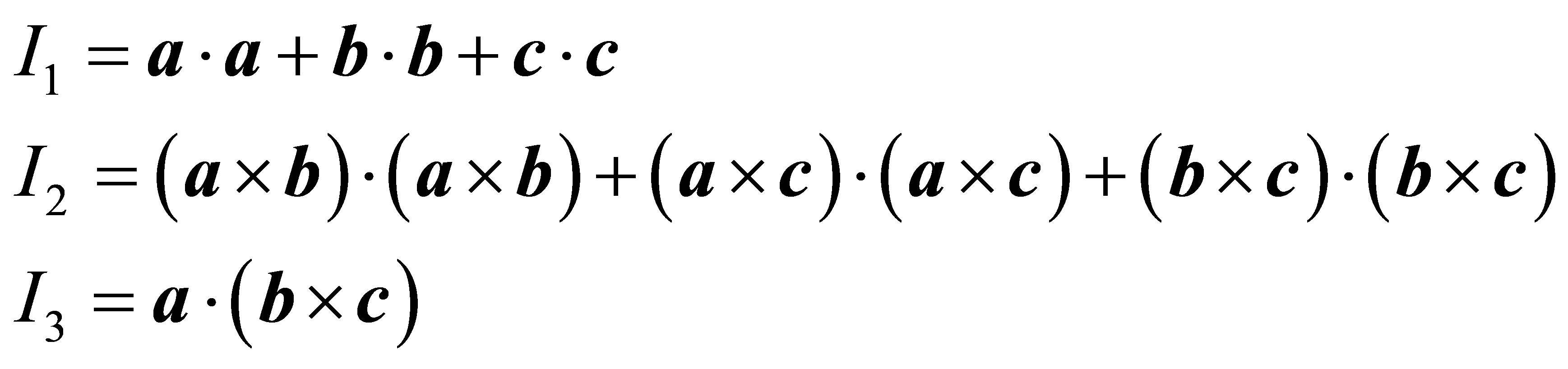 (6)
(6)
where ,
,  , and
, and  are the column vectors of
 .
.
The invariants for anisotropic bodies can be the six values produced by a Gram-Schmidt QRDecomposition of . This QRDecomposition results in an upper triangular matrix,
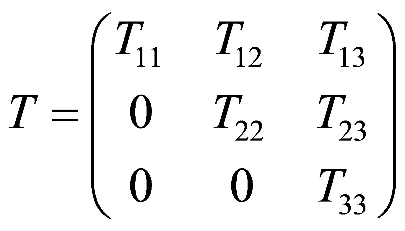 (7)
(7)
The elements of this upper triangular matrix can also be written in terms of the column vectors of  as follows:
 (8)
(8)
Any algebraic combination of these 6 values can also be used as invariants for anisotropic bodies.
2.2. Boundary Conditions
Boundary conditions for material deformation problems usually consist of either specifying the final positions of boundary points, or the forces on the surfaces. The Dirichlet boundary conditions consist of simply defining  at the desired surfaces. The Neumann boundary conditions require converting the surface forces into derivatives of
 . This can be accomplished by first noting that once
 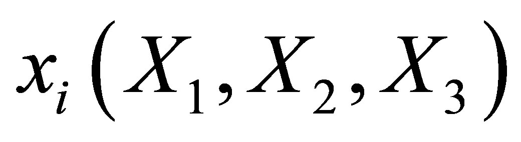 are known for a given deformation, E and
  are known. Thus the change in energy due to the work done on the body is a function of only the initial and final positions of the points within the body. This implies that the deformation forces are conservative. As a result the internal forces within the body can be written as the negative gradient of the energy,
  , which is equivalent to
 (9)
(9)
Care must be taken here, however, because the gradient of E is with respect to , whereas the integral is over the original
 . Using Equation (3),
 (10)
(10)
Applying the n-dimensional divergence theorem gives
 (11)
(11)
where  is the
  component of the force at the surface defined by the vector
  with
with ,
,  ,
, .
.
These internal forces must be balanced by an equivalent surface force in the opposite direction. Since this must be true for all surfaces, the surface forces  are
are
 (12)
(12)
Once the energy per unit volume, E, is expressed in terms of the invariants of , which are in turn functions of
 , Equation (12) provide the constraint equations for the Neumann boundary conditions.
3. Some Applications
The differential equations of elasticity have now been completely described. No reference has been made to the magnitude of the deformation. As a result, Equation (3) apply to both infinitesimal and finite elastic deformations. Also they apply to both isotropic and anisotropic materials. Although the equations are general, for simplicity I will limit the rest of this paper to isotropic materials.
3.1. Infinitesimal Elasticity
In order to make the connection between the differential equations of elasticity given here and the “standard” differential equations of infinitesimal elasticity, I will show that a Taylor expansion of  for an isotropic body yields the infinitesimal free energy as described by Landau [5] (Equation 4.1, p. 9). This infinitesimal free energy when substituted into Equation (3) results in the differential equations for infinitesimal deformations that Landau derived assuming strain to be the independent parameter.
The Taylor expansion of 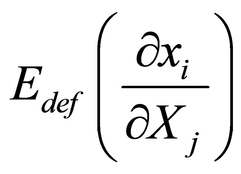 yields
 (13)
(13)
where the “0” subscript corresponds to no deformation (i.e. when  and
and ).
).
The first term in the expansion is a constant and is physically irrelevant. To evaluate the second term, I will choose to define the initial state, when no deformation has occurred, as corresponding to the state of the body when all internal forces are zero. Since this must be true for all points within the body, Equation (11) gives
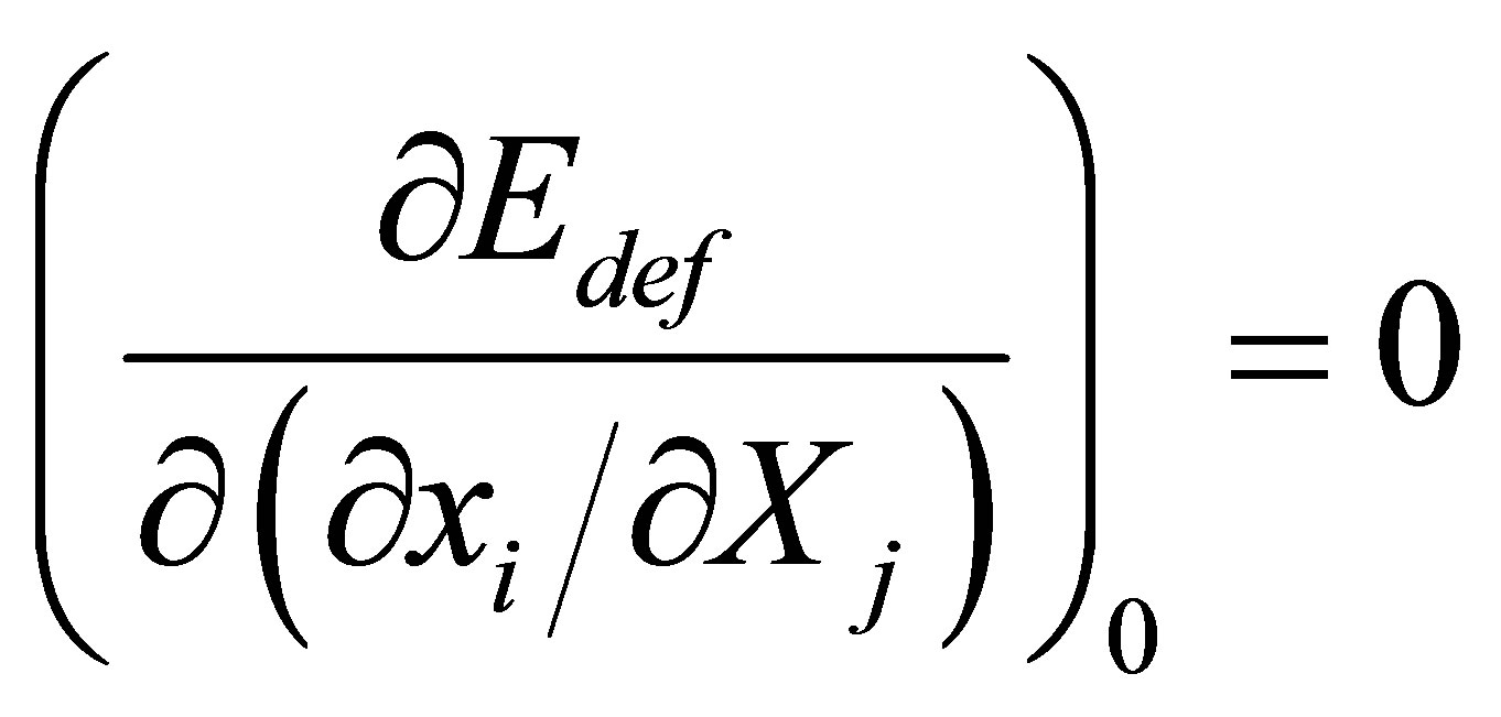 (14)
(14)
which is the coefficient of the second term in the Taylor expansion, Equation (13). As a result, the third term, is the leading term in the Taylor expansion. Before evaluating this however, let’s see what constraint Equation (14) provides. To do this, express  in terms of the three
  invariants for an isotropic body given in Equation (6) Then
 (15)
(15)
Direct substitution of the  invariants in terms of
  into this equation yields
 (16)
(16)
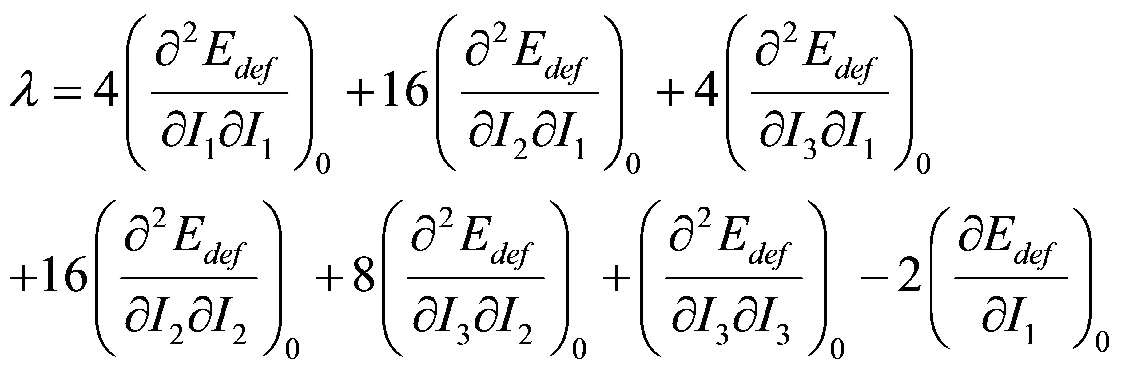
It now remains to expand and evaluate the third term in the Taylor expansion. Again writing  in terms of
  allows us to proceed. The third term in the Taylor expansion can be expanded quickly using algebraic computation software like Mathematica. It is a bit more tedious by hand, but the result of either is the free energy
  as defined by Landau [5],
 (17)
(17)
with  and
and , so that
  where
where
 (18)
(18)
and
 (19)
(19)
If this Taylor expansion of  is substituted into Equation (3) and a gravitational body force
  is added, we get Landau’s equation [5] (Equation 7.1, p. 16) of equilibrium for isotropic bodies of an infinitesimal deformation:
 (20)
(20)
where Young’s modulus  and Poisson’s ratio
 .
.
The boundary conditions for classical infinitesimal elasticity consist of setting stress and strain on boundaries. To complete the comparison, stress and strain need to be defined. There are many different definitions of stress and strain in the literature. As an example, the Lagrangian strain tensor is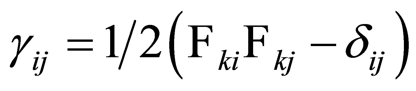 , and stress as defined by Landau [5] can be inferred from Equation (12) to be
 (21)
(21)
Note that this stress corresponds to force divided by original area. We can now conclude that all of the solutions to problems in classical infinitesimal elasticity described by Equation (20) are also solutions of Equation (3).
One other observation should be made here. As defined by Landau,  defined in Equation (21) is the stress exerted by the surroundings on the material volume. Noting this and considering the case where the material is in the gravitational field of the earth, we see that Equation (2) are just the equations of equilibrium
  in terms of stress, i.e.
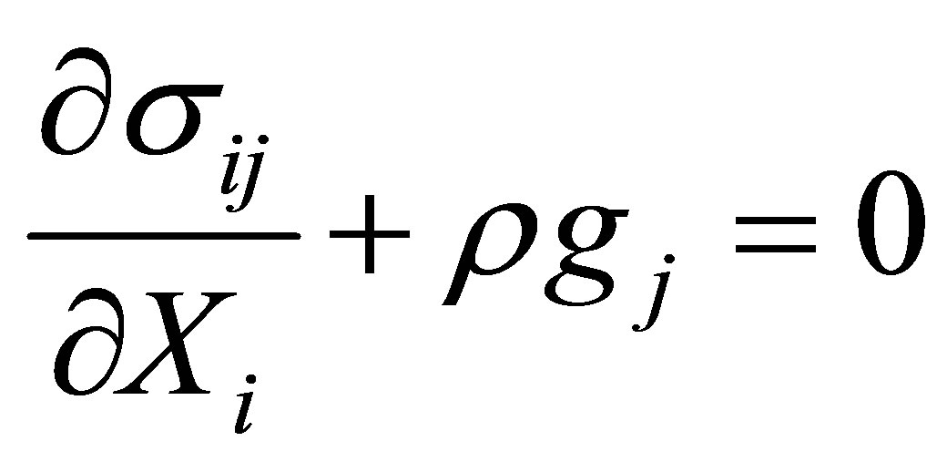 (22)
(22)
where .
.
3.2. Finite Elasticity
The real power of Equation (3) is not that they can reproduce standard infinitesimal elasticity equations, but that they apply equally well to finite elasticity. Consider for example a finite deformation with no body forces.
Since E is a function only of , the derivative of E in Equation (3) results in equations with every term containing a second derivative of
  with respect to
 . As a result, any homogeneous deformation without body forces automatically solves Equation (3), depending only upon the boundary conditions.
Consider two such homogeneous deformations. The first homogeneous deformation simulates the experimental results of Rivlin [6]. These experimental results can be used to define an energy function E. The second homogeneous deformation uses this energy function to calculate the surface forces necessary to produce a simple shear of 25˚, which is much larger than would be possible with infinitesimal elasticity theory.
3.2.1. Matching Experimental Data
Any of the many models of elasticity expressed in terms of invariants of  (e.g. Ogden [3]) can be used for
  in Equation (3) as long as they span the range of deformation conditions to be encountered in the simulation. As a specific example, consider
  given as
 (23)
(23)
Note that the coefficient of  has been chosen so that Equation (16) is satisfied (i.e. so that the forces with no deformation are zero). Considering solutions of Equation (3) of the form
 , the deformation gradient matrix is
 (24)
(24)
and the singular value decomposition of  gives
gives .
.
 ,
,  ,
,  , and
, and  were measured by Rivlin. No force was applied in the z direction, so
 . Table 1 in Rivlin’s paper [6] recorded computed stress,
  where
where
 where w = original width = 8 cm, h =
original thickness = 0.7 mm of the deformed rubber sample. This information allows the measured  and
and  to be reconstructed. Substituting these
  values into Equation (12) provides three constrain equations for finding a, b,
  , and
, and . Unfortunately Rivlin assumed the rubber he deformed to be incompressible, so
  and b can not be evaluated using his data. However, if a,
  ,
,  are computed assuming incompressibility, an estimate of b can be obtained using compressibility
  from Wood [7],
  , Equation (18), and Equation (19). The result of this fit is
 ,
,  , c1 = 2.0902, c2 = −0.127399 all in Rivlin’s units of
 . Poisson’s ratio is 0.499888 and Young’s modulus is
 . These results are at least consistent with Rivlin’s data. The process followed here to derive
  is not ideal. What is really needed is experimental data for the entire energy cube as describe by Hardy and Shmidheiser [4]. Lacking that experimental data, I will use the energy function Equation (23) to demonstrate a case of finite simple shear.
3.2.2. Simple Shear
A simple shear, corresponding to a 25˚ deformation in the y direction, is ,
,  , and
, and . The forces required for this deformation on a cm cube can be found using Equation (12) and the energy function that fits Rivlin’s data, Equation (23). The result is
 ,
,  , and
, and  all in Newtons, with
 ,
,  , and
, and  being the force against what was the original yz, xz, and xy face, respectively.
Of course not all deformations are homogeneous, but Equation (3) are appropriate for finite element or any other technique for solving differential equations for more complicated problems when homogeneous deformations do not satisfy the boundary conditions of a particular problem.
4. Conclusion
Elasticity theory has been dominated by Cauchy’s stress and strain. Cauchy’s approach works well for infinitesimal elasticity as used in most engineering applications. For finite deformations, however, Cauchy’s approach becomes unduly complicated, spawning a number of new definitions of stress and strain. The Euler-Lagrange approach presented here avoids these complications. In addition, material properties in terms of the energy of deformation are easily input into the elasticity equations, Equation (3). It is my hope that engineers and physicists who require computer models of finite deformations will consider the Euler-Lagrange approach. I also hope that it will encourage experimentalists to “map out” the energy of deformation for more materials as Rivlin has done with rubber.
5. Acknowledgements
I would like to thank Jens Feder, Torstein Jossang, Richard Beier, Paul Meakin, and Jonathan Gaston for their support and encouragement of this work.