Identification of Water Quality Model Parameter Based on Finite Difference and Monte Carlo ()
1. Introduction
In order to allocate water resources rationally, many Long Distance Water Transfer Projects (LDWTPs) have been built or are being constructed in China. But there are numerous controls and cross buildings along the process in LDWTP, so it is highly possible that sudden water pollution incident happens [1]. Once these incidents occur, it is necessary to reveal the rule of pollutants transport and diffusion based on water quality parameters quickly, and then put forward emergency disposal counter measures, otherwise it will cause inestimable consequences [2]. Therefore, it is crucial to identify water quality model’s parameters. Many approaches have been proposed to identify the parameters of water quality model, such as theoretical formula method, empirical formula method and tracer test method, etc. [3]. The tracer test method belongs to the category of inverse problems which include methods such as moments, fitting, optimization and the uncertainty analysis [4]. With the development of computer technology, identification method based on Optimization has been widely used, such as Simplex method [5], Particle Swarm Optimization [6] et al. But there are many strict limit conditions and the non-identificability will increase with the increase of parameters’ number when using these methods. In addition, LDWTP is complex and giant system, in which there are full of uncertain factors, and it don’t exist analytical expressions of pollutant concentration. Therefore, it is necessary to find a better identification method to research the rule of pollutants transport and diffusion in LDWTP.
Therefore, a new method which named FDM-MCMC is proposed based on Finite Difference Method (FDM) and Markov Chain Monte Carlo (MCMC) in this paper to identify the water quality model parameters. And in order to verify this proposed algorithm’s accuracy, efficiency and anti-noise capability, the results of parameters identification with different scenarios are analyzed by numerical simulation. Finally this proposed method is compared with Finite Difference Method and Nelder Mead Simplex (FDM-NMS).
2. Materials and Methods
2.1. Description of the Problem
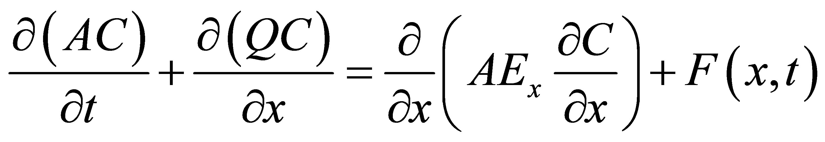
LDWTP is a series system consists of many canal pools which are divided by gates, as shown in Figure 1 [7]. If pollutants in canals are attenuated by the first order kinetics, the law of pollutants’ transportation and diffusion is described by:
 (1)
(1)
where A is cross section area, C is the concentration of pollutant, Q is cross section flow, t is the time, x is the longitudinal coordinate, Ex is the longitudinal dispersion coefficient, F(x, t) is the source term.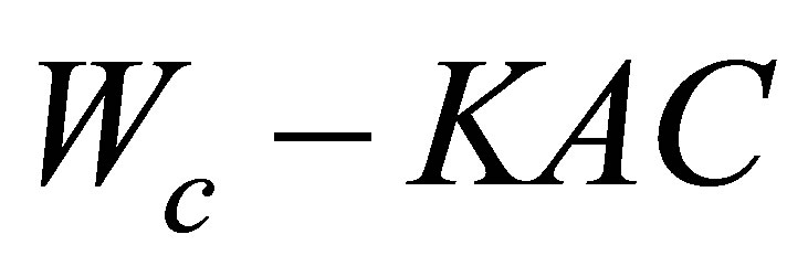
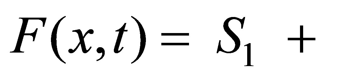 , S1 is internal source (sink), K is reaction rate, Wc is the exogenous input terms.
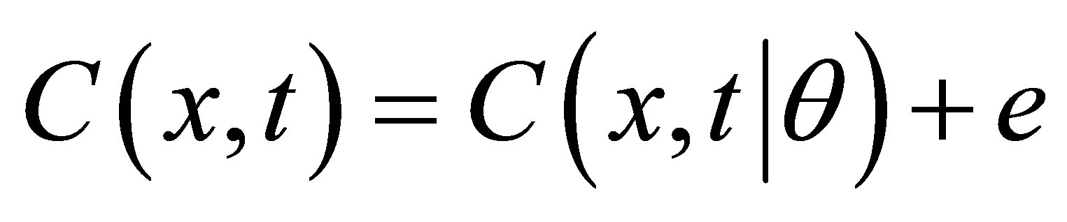
According to Figure 1, LDWTP is a complicated nonlinear system and the concentration of pollutant can be expressed as:
 (2)
(2)
where θ is a set of parameters set, which is difficult to be measured. And the concentration of pollutants is on the section of canal pool (see Figure 2).
According to Figure 2, Equation (1) can be transformed into (3) [5]:
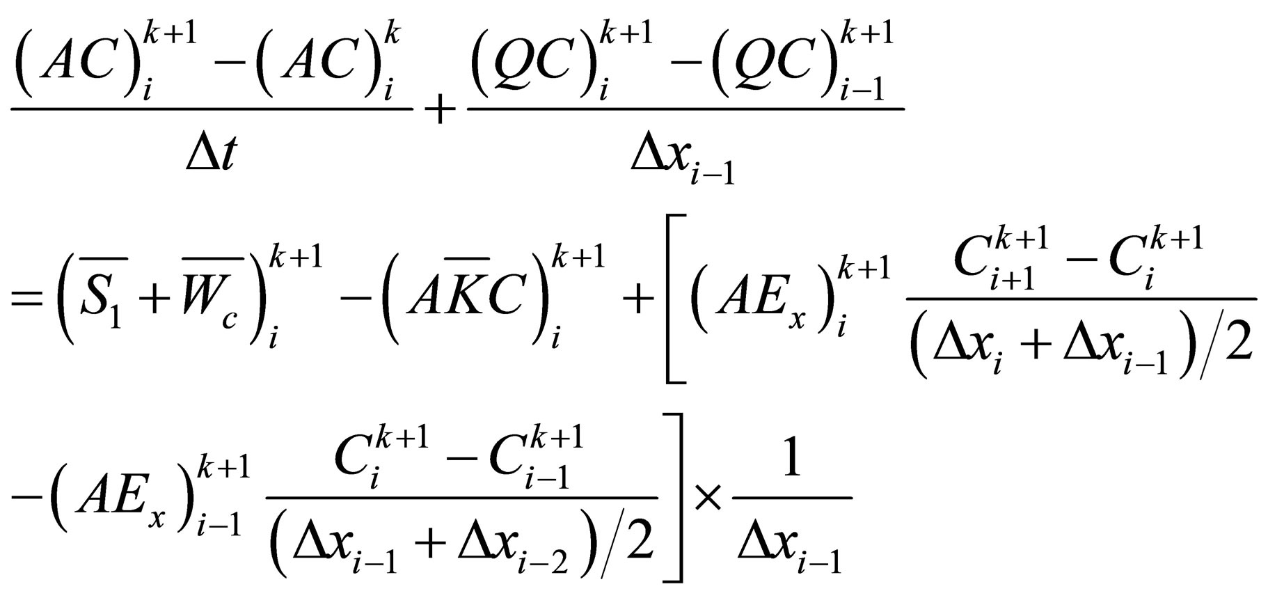 (3)
(3)
where  is the pollutant concentration of the ith canal pool at k + 1 moment, so Equation (3) can be expressed as:
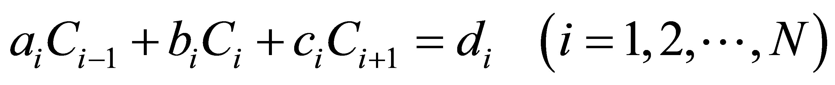 (4)
(4)
where ai, bi, ci are coefficients; di is a constant. Equation
(4) is a linear implicit difference equation which is made up of N equations and it can be solved by combining with the upstream and downstream boundary conditions.
Therefore, the identification problem of water quality model parameters in LDWTP can be solved by a limited concentration measurement data. However, since the uncertainty of the model structure and the observation data, the FDM-MCMC method is developed to solve this problem.
2.2. Methods
Uncertainty identification method based on the Bayesian theorem can avoid the decision risk caused by the distortion of the “optimal” parameters in a certain extent [8]. So according to Bayesian theorem, it can be stated as follows:
 (5)
(5)
where θ is the unknown parameter; y is the observed data; p(y|θ) is the likelihood function; p(θ|y) is the parameter’s posterior probability density function; p(θ) is the parameter’s joint priori probability density function.
Assuming  is the measurement error, ei is the prediction error, and these errors are independent and obey Laplace distribution. So the problem of model parameters can be transformed to solve the parameters’ posterior probability density function:
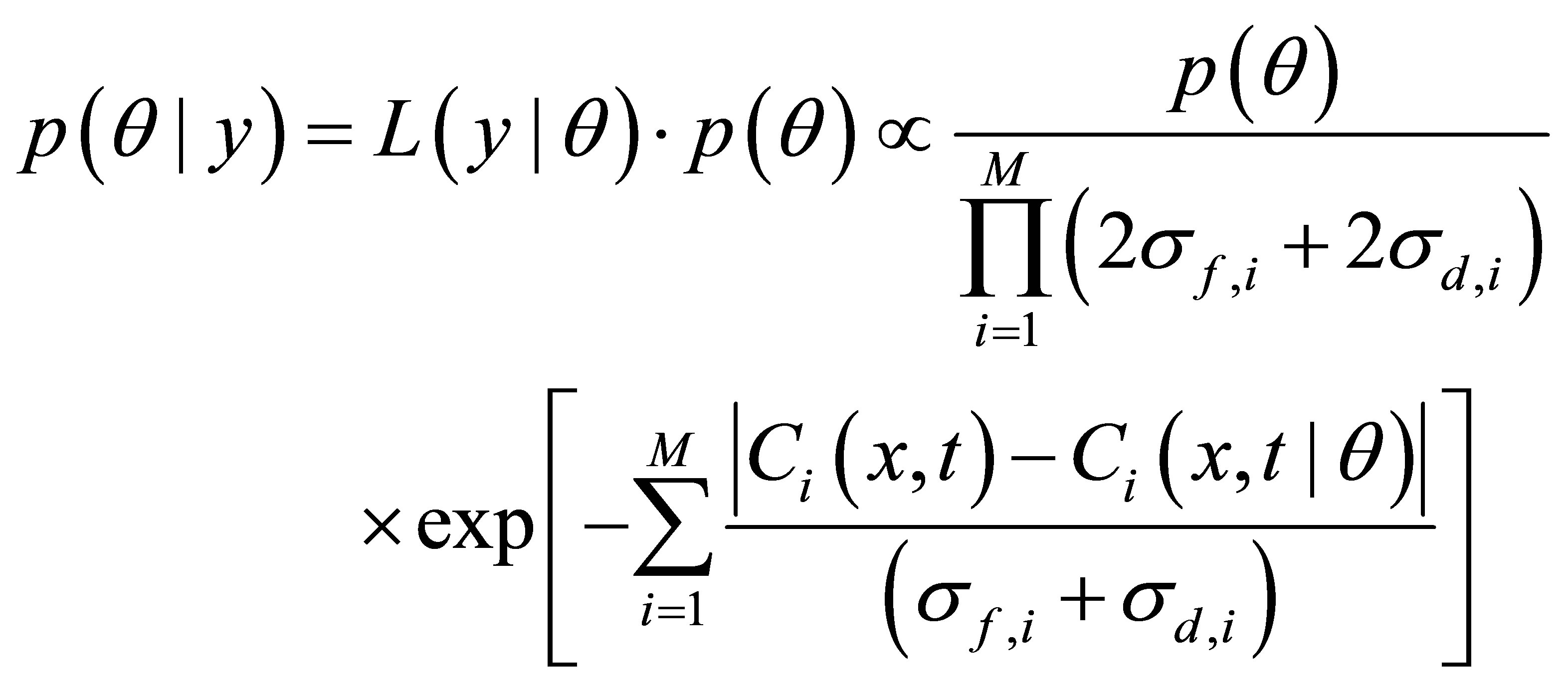 (6)
(6)
where M is the number of observation data, σd,i, σf,i are the standard deviation of εi and ei, respectively.
Therefore, the estimated values of the unknown parameters can be obtained by Equation (6) and MCMC method which is based on sampling random method. Since Metropolis-Hastings is a sampling method in a generation-rejection sample forms, a new identification method based on Bayesian-Markov Chain Monte Carlo to
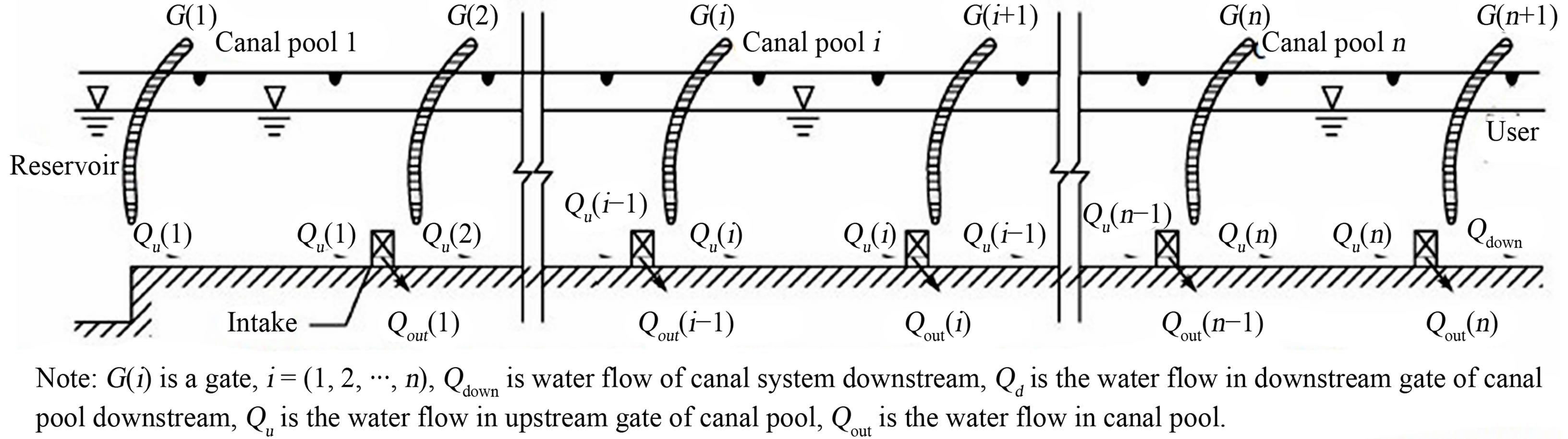
Figure 1. Sketch of the controlled canal system.
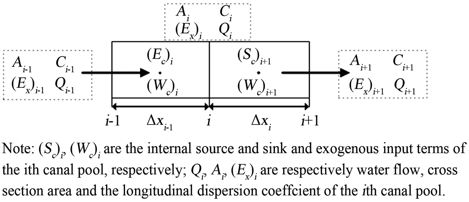
Figure 2. The finite difference format to the wind of water quality model equation.
identify the parameters in this paper [9]. The detailed solving steps are as follows:
1) The study area is divided into N canal pools by spatial discretization and each canal pool section has only a little change over time and space;
2) Determining sample space and p(θ(i)) of the unknown parameters;
3) Generating initial values θ(i)(1), θ(i)(2),···, θ(i)(S);
4)Obtaining the conditional probability density by setting the Proposal distribution q(θ(i)(S), θ(*)(S)), generating θ(*)(S), and calculating the θ(i)(S) and θ(*)(S) corresponding to the pollutant density;
5) Finding the likelihood function which can reflect the relationship between the model parameters and measurement data, and then calculating the posterior probability density function;
6) Getting the accept probability A(θ(i), θ(*)) at which Markov Chain moves from θ(i) to θ(*) as following [9]:
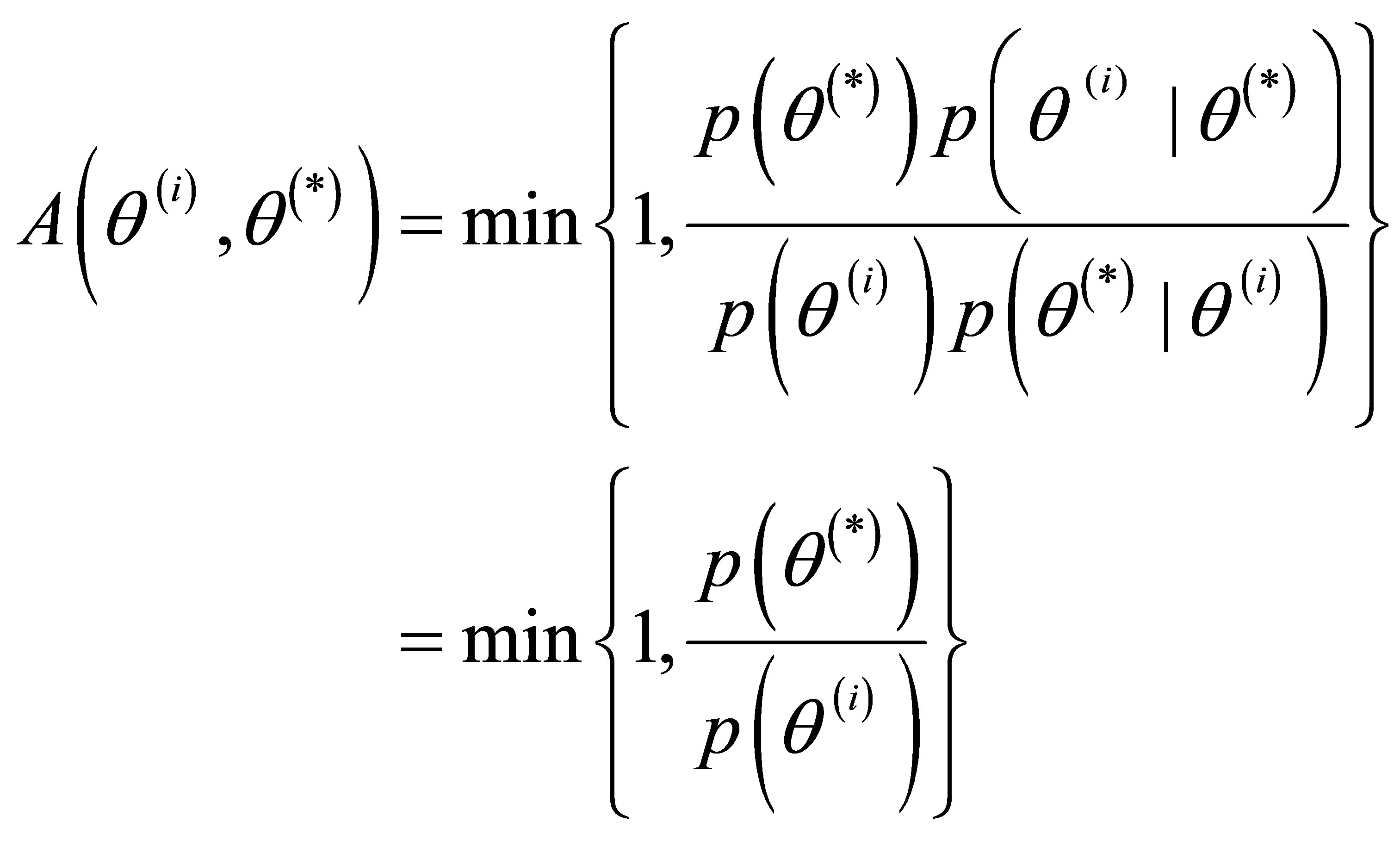 (7)
(7)
7) Generating a random number which belongs to 0 - 1 and obeys uniform distribution. If R < A (θ(i), θ(*)), then setting θ(i+1) = θ(*), otherwise, θ(i+1) = θ(i);
8) Repeating steps from 1) to 7) until it reaches a predetermined iterations.
3. Results
For LDWTP, the “twin” experimental is an effective means to identify parameters of water quality model [10]. However, the longitudinal dispersion coefficient is becoming more and more important in the sudden water pollution accident [11]. Therefore, an open channel with 3km length is taken as an example in this paper. Assuming the inflow water concentration in the upstream (x = 0) is 1.0 mg/L and free outflow in downstream. The flow field distribution is u = 0.5 + 0.001x and the channel can be dispersed into N = 6 canal pools according to the channel’s geometry features whose true values of longitudinal dispersion coefficient (Ex)i (i = 1,···, N) are 50, 70, 90, 110, 130 and 140 m2/s.
3.1. Steady Non-Uniform Flow
Assuming flow Q is equivalent to 10 m³/s, and then the identification results are obtained as error level σ = 0.1 by using FDM-MCMC and FDM-NMS method, respectively, as show in Table 1.
From Table 1, while σ = 0.1 the average relative error obtained by FDM-MCMC and FDM-NMS method are respectively 4.99% and 8.25%.
3.2. Unsteady Non-Uniform Flow
If the flow of this open channel is a function of time, it is Q(t) = 10 + 0.001t, the identification results of obtained by FDM-MCMC and FDM-NMS under different noise are shown in Table 2. Here we take relative standard deviation (RSD) as the accuracy of the identification values:
 (8)
(8)
where λ is standard Deviation; μ is the mean of identification value. So when σ = 0.1, RSD obtained by the two methods are shown in Table 3.
From Table 2, the average relative errors are respectively 3.41% and 8.26% by FDM-NMS and are respectively 2.93% and 5.14% by FDM-MCMC. From Table 3, the average RSD is respectively 27.30% and 52.96% by FDM-NMS.
4. Discussion
Therefore, comparing with FDM-NMS, the FDMMCMC has the following advantages:
1) Wider applicability
In the two scenarios, When σ = 0.1, the average relative errors are less than 6% by the FDM-MCMC. So the FDM-MCMC has strong applicability. It is not only ap-
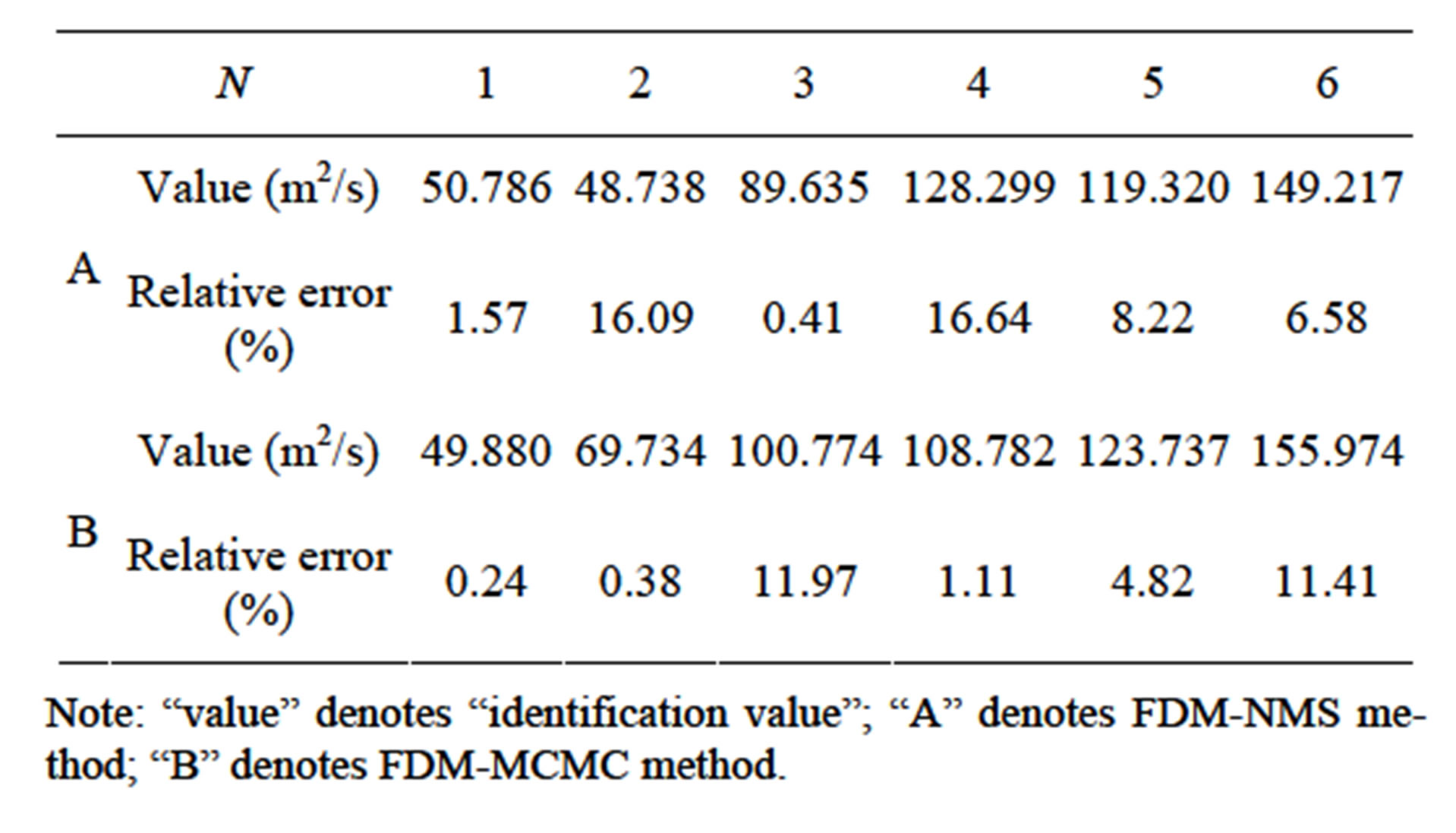
Table 1. Identification results by FDM-NMS method.
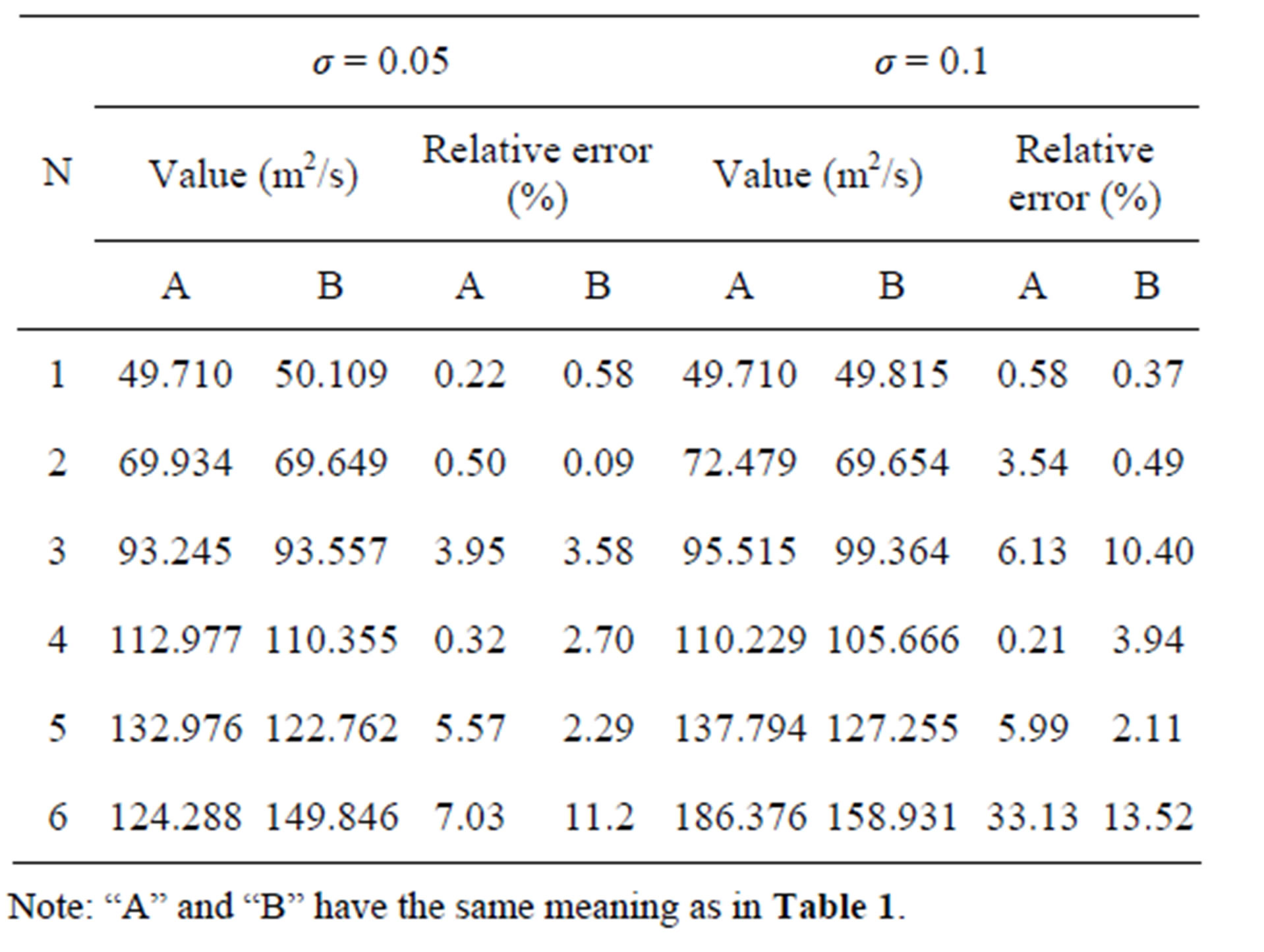
Table 2. Identification results by FDM-NMS method.
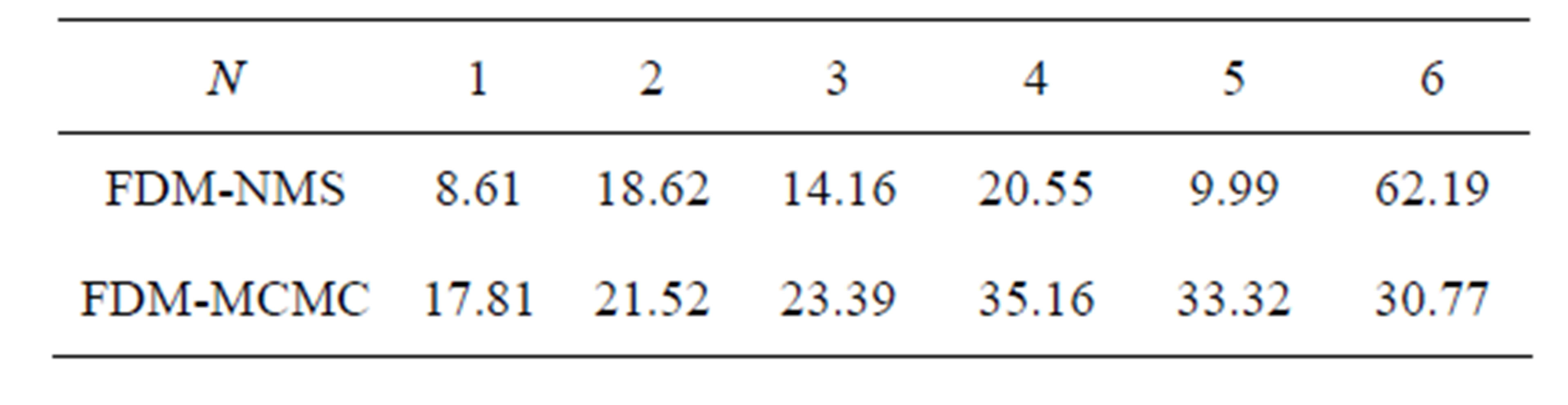
Table 3. RSD of identification value by the two methods %.
plicable to the constant flow, but also applicable to the unsteady flow.
2) Higher accuracy The average errors by FDM-MCMC are less than by FDM-NMS method, which are respectably 3.26% and 3.12%. So the precision of identification results by FDMMCMC are higher than by FDM-NMS in the same circumstances.
3) Stronger anti-noise ability The average relative errors obtained by FDM-NMS and FDM-MCMC method are both less than the corresponding measurement errors. But the average relative standard deviation obtained by FDM-MCMC is less 25.96% than by FDM-NMS.
In summary, the FDM-MCMC has wide applicability, high identification accuracy and anti-noise ability. It can be better to identify the parameters of water quality model in LDWTP.
5. Conclusion
With the improvement of water quality model function, the identification difficulty is becoming more and more. Therefore, the Finite Difference Method is adopted to solve water quality model in LDWTP, then based on the Bayesian inference the unknown parameters’ posterior probability density function is identified, and further the corresponding statistics are obtained by sampling with MCMC to identify water quality model parameters in LDWTP. According to the numerical results, it improves significantly not only on the global convergence and convergence rate, but also the identification accuracy is relatively higher by the FDM-MCMC in solving water quality model parameter identification problem with higher nonlinear degree. Because the FDM-MCMC has the characteristic of strong targeted to improve, it is applicable to other nonlinear identification problem. In addition, it will cause large amount of calculation for the large required sample number. So as to reduce the computational complexity greatly, combing with other inversion methods and making it possible to apply in real-time identification mode would be the future research direction.
6. Acknowledgements
The research work was supported by the national science and technology major special project (No.2012ZX 07205005) and the public welfare industry research project of the ministry of water resources of the People’s Republic of China (No.201101063).
NOTES