Functional Enrichment of Utopian Distribution of Plant Life-Forms ()
1. Introduction
Plant life-forms are a primary means by which to categorize forms of plant growth, together with life history strategies and metabolism. Life-forms are an effective way to show distribution of plant species on a macro scale with use of computational statements [1,2]. Patterning of plant species may be determined by key factors of the water-energy dynamic [3-5]. Climatic variables such as rainfall and temperature often show discrete patterns across timescales, so are often made use of within fixed time ranges. As such, they can be said to be discrete stochastic patterns, which facilitate macro-level modelling of plants [6-8].
Utopian distribution refers to the informative combined objective Z matrices, which may be generated through the use of techniques including adaptive fuzzy neural inference systems, genetic programming, and particle swarm optimization [9-13].
Functional relations may be explored within the products of evolutionary algorithms via the use of functional process models, which may display continuous or discontinuous qualities [14,15]. Computational methods may be applied to differentiate biological systems such as reservoir capacity for life, environmental indices [8,16, 17].
There are five main groups of life-forms: phanerophytes, chamaephytes, hemicryptophytes, cryptophytes and therophytes. Within the main groups there exist a total of 18 subgroups, with the following characteristics: Phanerophytes are of three types: 1) evergreen phanerophytes with bud scales; 2) evergreen phanerophytes without bud scales; 3) deciduous phanerophytes with bud scales. Phanerophytes are further divided according to height: Mega-(>30 m); Meso-(8 - 30 m); Micro-(2 - 8 m); Nano-(<2 m).
Chamaephytes have woody and herbaceous types. Chamaephytes are broken into: 1) Suffruticose- (after the main growth period upper shoots die, only lower parts of the plant remain in “unfavourable” period); 2) Passive- (in unfavourable conditions upper shoots become procumbent, protecting them from environmental stresses); 3) Active—(shoots only produced along the ground and remain so); 4) Cushion—(similar to passive type but shoots are so closely packed together they form a “cushion”).
Hemicryptophytes are further divided into: 1) Proto- (leaves are well developed up the stem of the plant, partially developed leaves protect growing buds); 2) Partialrosette—(developed leaves form a rosette at the base of the plant, the following year a long aerial shoot may grow); 3) Rosette (leaves restricted to a basal rosette, long exclusively flower bearing aerial shoot forms).
Cryptophytes are divided into: 1) Geophyte—(underground organs such as bulbs, rhizomes, tubers, shoots emerge in growing season); 2) Helophyte (growing buds are in soil or mud under water producing shoots above water); 3) Hydrophyte—(buds lie under water, unfavourable period spent completely below water).
Therophytes are annual plants, which survive the unfavourable period as seeds, completing their life cycle in the summer months.
Life-forms are often seen in differing proportions or spectra; plants show chaotic patterns of evolution in terms of their individual growth processes and numbers [18-20]. Life-form differences are often associated with variable gradients in topographical and climatic conditions [21,22]. In order to clarify the difference in lifeform spectra this study considers two contrasting areas known to be rich in plant numbers: Ecuador, South America and Macedonia, Southern Europe [23-26]. The former of these has been well documented as being the most diverse location on the planet and the latter has previously been algorithmically defined as having the characteristics of a more extreme environment (elevated temperature, comparatively low rainfall).
In this paper proportions of plant life-form characteristics are investigated within fixed population sizes, which have been determined from a combined genetic algorithm fuzzy rule base, furthered by field based studies [24,26].
The aim of this study is to identify the functional approximation algorithm using the following steps: Geographic and climatic study to establish the framework for modelling species of plant life-forms in candidate areas; adaptive fuzzy neural inference system (ANFIS) using identified variables based on consequent primary nodal number; multi objective genetic algorithm dispersing expanded secondary nodal number; functional approximation of characters within secondary nodal number using a continuous/discrete surrogate process model.
2. Methods
In this section we describe the steps of our functional approximation algorithm. Elements of the methods are presented in [27,28]. Definitions are given within the following sections further details of which can be found in [9,15,17,29].
2.1. Digital Elevation Model and Climatic Data Sourcing
Climatic areas of diversity zone 8 - 10 [23], documented as containing greater than 3000 species per 10000 km2, were investigated and given algorithmic definition [30]. Further these areas are included within high resolution mapping tiles available from the Intergovernmental Panel on Climate Change (at 18.5 km resolution) and the United States Geological survey (at 1 km resolution). Two candidate areas were selected from the literature to show the breadth of difference in climatic, topographic and actual documented numbers of individual plant occurrences within the areas. The selected areas were Ecuador, including the reserve surrounding Tiputini Biodiversity Station there (covering approximately 10,000 km2) [24,31] and the country of Macedonia (covering 25713 km2 (European Environment Agency, http://www.eea.europa.eu/ accessed 30 06 13)). Coordinates for each area were obtained from the above sources and verified after investigation (via the IPCC and USGS web site) using the technical computing platform Matlab (Version R2010a ©). Coding was constructed in Matlab (available on request) enabling display of the digital elevation model (DEM), precipitation, temperature and ground frost frequency data for each region. Variables are quantified to maximize computational efficiency and interpretability of the ANFIS. The structure of ANFIS is given in Section 2.2.
2.2. Adaptive Neural Fuzzy Inference System Structure
ANFIS is commonly built using Takagi-Sugeno-Kang (T-S-K) or Mamdani fuzzy logic. T-S-K fuzzy systems [32,33] are more easily applied to multiple input and multiple (ranged) output. The general form of the ith rule as applied to T-S-K systems is as follows:
 (1)
(1)
Here we see a constructive breakdown of the antecedent term A, which may be dispersed through multiple sets of linguistic variables such as those present in climatic systems. These are detailed as:
 (2)
(2)
where  are set values of generic set X. Additionally the following definitions using multiple elements in T-S-K systems are applied:
 (3)
(3)
 (4)
(4)
 (5)
(5)
In (3) the mean of set x is represented by normal set elements . Accordingly, (4) the mean of set y is represented by normal set elements
 . In (5) fA refers to function A in x and Xµ is the grade of membership of X and may also be used to express function A in y and Yµ is the grade of membership of Y. Both X and Y are used in the antecedent linguistic A in order to form:
 (6)
(6)
where R is the relational index as a function of the combined arguments of  and
and  or succinctly defined as “IF A··· THEN B” [33].
Given the above definitions, the nodal structure of an ANFIS engine is developed with the insertion of crisp input variables (A1(1,···, n),··· An(1,···, n)) in the first layer; membership function [0,1] fuzzifies the crisp inputs in the second layer; If (antecedent) Then (consequent) rules operate in the third layer; output membership function [0,1] operate in the fourth layer; summation of the output membership layer (defuzzification) and conversion back to crisp values give the output of the engine. One may then summaries the ANFIS via algorithmic statements detailing the rules linguistically. Partitioning of the membership functions interval is crucial in fuzzy systems. In this study the variables are given 5 partitions within the membership function, which ordinate the crisp inputs via triangular functions [9]. Parameters (mean and variance) are defined according to:
 (7)
(7)
where parameters a, c are the feet and b are the peaks. The structure of the algorithm therefore appears as follows:
 (8)
(8)
where A(1),··· A(n) are antecedent singletons, (e.g. Temperature, precipitation and altitude) and B(n) is the consequent environment (E) given by the number of individual plant species occurrences (sourced from the Global Biodiversity information facility (http://gbif.org accessed December 2012) as validated by [34]). ANFIS were built using Matlab (Version R2010a ©) and code is available on request.
2.3. Multi Objective Genetic Optimization Selection and Dispersal of Elements
Genetic algorithms (GAs) are adaptive algorithms for finding the best (global) solution to optimization problems. The stages of GA are as follows: start with a population of randomly generated “chromosomes” (not actual chromosomes but sequences of defined length); initialisation, the collection of “chromosomes” (sequences) evolve through a form of natural selection. Each iteration of selection is known as a generation, and the chromosomes are rated for their “adaption for solutions” or potential to solve the problem. On the basis of the evaluation, a new population of sequences is formed using a process of selection. At this point, genetic processes analogous to crossover and mutation take place. After further selection, given the solution is found an output is given. Evaluation or fitness function must be devised for each problem to be solved. Given a particular sequence or chromosome solution, the evaluation function returns a single numeric value proportional to the adaptation of the solution represented by the chromosome or sequence [35].
In this paper the initial number of 5 plant life-forms is expanded to cover the complete number of 18 sub-groups of life-forms, each sub group being quantified within an interval [1,5]. Code is constructed (available on request) in Matlab to enable the random, tournament selection spacing of each of the elements of life-forms within a combined objective axis, demonstrating the distribution of the elements in Z (utopia) space as a Pareto front. Plotting linear and varying degrees of polynomial regression through the Pareto front enables precise statements to be made. One can extrapolate values of the objectives [36] enhancing the accuracy of measurement of the original antecedent variables, which in the current case are climatic measurements. The consequent variable (numbers of plant species) is also enhanced. This process is carried out for contrasting locations with different numbers of plant species in order that the variance of opposing areas may be compared. A location ideal for plant growth (Ecuador, South America) and a more extreme drier area (Macedonia) are compared in this study.
2.4. Functional Approximation Algorithms Using Surrogate Models
We proceed with a further method of generating the Z matrix via the use of a surrogate function. We made the assumption that individuals within the populations of plant species in each of the studied areas are normally distributed in their life-form characteristics. Additionally standardization of the dispersed Strength Pareto population to zero mean and unit variance allows the population to be expressed across a bell shaped (Gaussian) curve [37].
In our choice of Gaussian models we selected Rastrigin’s function, which served the dual purpose of expanding the dispersal of the 18 sub groups of lifeforms simultaneously and verified the validity of the GA process described in Section 2.3. (Code for the Rastrigin’s function as applied to 18 life-form sub groups in Matlab (Version R2010a ©) is available on request).
 (9)
(9)
where i = 1/n, xi is an element of the interval [−5.12, 5.12]. Life-form categorization occurs within the interval shown.
3. Results
We present the implementation of steps 1 - 4 towards formation of the functional approximation algorithm here. Section 3.1 shows topographic mapping of GTOPO30 for Macedonia and then for Ecuador. Climatic data [7] used for modelling of the water-energy dynamic are also exemplified. Section 3.2 details the rule structure for each and shows the algorithmic structure as applied to plant life-forms, exemplifies the building of the ANFIS, and gives additional examples of the 3 dimensional surface view of the algorithms. Section 3.3 includes the quantification of sub-groups of plant life-forms and shows the objective dispersal of the Strength Pareto Evolutionary population obtained, and gives linear and quadratic expressions by which the accuracy of objective functions and consequent values are enhanced. Finally, Section 3.4 shows extrapolation of life-form groups across the Z utopia hyperplane using the functional approximation algorithm.
3.1. DEM and Climatic Data
The data presented in this section exemplify those that may be used to form fuzzy algorithms, and on which we operated a genetic (generational) structure. We successfully predicted water-energy objective dispersion of plant species [30]. Topographic data are quantified in Table 1 and climatic variables are quantified in Table 2. Should further detail be required contact the first author. The areas covered are 1) mainland Ecuador, South America which falls in between northernmost latitude 1.464504 degrees, southern most latitude −5.02194 degrees and easternmost longitude −75.19056 degrees, westernmost latitude −81.023841 degrees and 2) Macedonia, southern Europe, which falls in between latitude 43 degrees north, 40 degrees north and longitude degrees 20 east, 23 degrees east. Coordinates of the locations were obtained using United States Geological Survey (USGS) data and extracted using Matlab (version 2010a ©) and validated by [24,31], (European Environment Agency, http://www.eea.europa.eu/ accessed 30 06 13).
The DEM data of GTOPO30, published through the United States Geological Survey (USGS), are shown graphically in Figure 1. They are at 30 s (1 km resolution). Data were processed using Matlab (version R2010a ©). Code was constructed for mapping and image-processing sections of Matlab and is available on request.
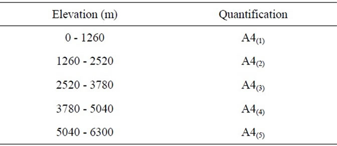
Table 1. Quantification of DEM data.
In Figure 1 Ecuador shows an elevation range from 0 m to 6300 m above sea level, whereas Macedonia shows an elevation of 0 m to just over 2520 m above sea level.
The elevation ranges of Ecuador and Macedonia were quantified according to a five-split partitioning of the range as shown in Table 1.
In Figure 2 Ecuador shows temperatures of −3 to >21 ˚Celsius in January, April, July and October; Macedonia shows temperatures of −27 to 21˚Celsius in January, −3 to 21˚Celsius in April, 21 to 45˚Celsius in July, and −3 to 21˚Celsius in October. Temperatures were quantified according to the method shown in [30].
In Figure 3 Ecuador shows precipitation of 0 - 500 kg m2 in January, April and October and 0 - 400 kg∙m2 in

Figure 1. Digital elevation maps for (a) Ecuador, South America; (b) Macedonia, Southern Europe.
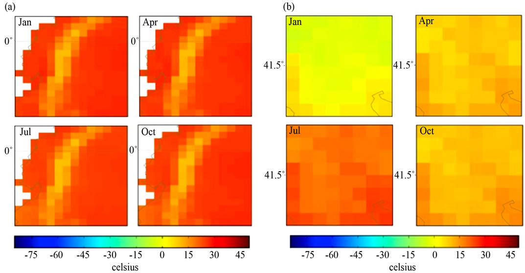
Figure 2. Quarterly mean temperature (1961-90) of (a) Ecuador, South America and (b) Macedonia, Southern Europe.
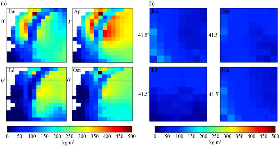
Figure 3. Quarterly mean precipitation (1961-90) of (a) Ecuador, South America and (b) Macedonia, Southern Europe.
July. Macedonia shows precipitation of 0 - 200 kg∙m2 in January, April and October and 0 - 100 kg∙m2 in July. Data of ground frost frequency [7] is available on the IPCC web site. All climatic variables are displayed at 18.5 km resolution. The method for quantification of climatic variables is shown in [25]. Temperature was designated as A1, precipitation as A2, ground frost frequency as A3 and elevation as A4 to enable the construction of the ANFIS engines, which is detailed in the following section.
3.2. Construction of the ANFIS Engines for Ecuador and Macedonia
After quantifying the variables for the geographic locations of Ecuador and Macedonia, and sourcing the number of individual plant occurrences from the Global Biodiversity Information Facility (http://gbif.org, accessed December 2012), the following concise fuzzy singleton antecedent-consequent rule bases were applied in order to build the inference engines:
 (10)
(10)
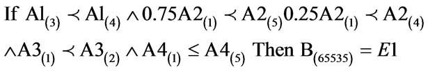
The above algorithm translated into the following conditions: IF Variables (A) = Temperature = 60% - 80%; Precipitation = 0.75 × 0 - 100 kg∙m2 to 400 - 500 kg∙m2, 0.25 × 0 - 100 kg∙m2 to 200 - 300 kg∙m2; Ground Frost Frequency = 0 - 6 days to 6 - 12 days; Altitude = 0 – 6300 m THEN Environment 1 (Phanerophytes dominant ≤ Chamaephytes ≤ Hemicryptophytes ≤ Cryptophytes ≤ Therophytes) (B) = 65535 individual plant occurrences. (10) Creates 17 rules with variable weights as shown in Table 2.
The terms Low, Low-Medium, Medium, Medium, Medium-High, High are quantified according to [25].
(11) Shows the algorithm for Macedonia.
 (11)
(11)
The above algorithm translated into the following conditions: IF Variables (A) = Temperature = 0.25 × 60% - 80% to 80% - 100%, 0.5 × 60% - 80%, 0.25 × 80% - 100%; Precipitation = 0.75 × 0 - 100 kg∙m2 to 100 - 200 kg∙m2, 0.25 × 0-100 kg∙m2; Ground Frost Frequency = 0.25 × 0 - 6 days to 24 - 30 days, 0.5 × 0 - 6 days to 6 - 12 days, 0.25 × 0 - 6 days; Altitude = 0 – 3780 m THEN Environment 5 (Hemicryptophyte, Therophyte dominant ≤ Chamaephytes ≤ Hemicryptophytes ≤ Cryptophytes ≤ Phanerophytes) (B) = 2023 individual plant occurrences. (11) Creates 16 rules with variable weights (further details available on request).
The first layer of the computational engine shown in Figure 4 accepts the crisp input variables, the second layer enables conversion of the variables according to their membership functions values/terms, the third layer is where the rules of the engine operate (seen in Table 2), the fourth layer converts the values back through membership function partitioned terms and the fifth layer computes the specific (crisp) number applicable for the predominant life-form type. The estimated primary consequent nodal number is 65535 (individual plant occurrences) for Ecuador and 2203 (individual plant occurrences) for Macedonia (GBIF (http://gbif.org, accessed December 2012) [34]).
The efficiency of each pair of variables may be seen viewing the surface of the algorithm. Clear definition is a good indication of accuracy achieved and helps us to choose which variables are minimized in optimization techniques [28].
Figures 5(a) and (b) show similar defined peaks of life-form differentiation, whereas Figures 5(c) and (d) give no defined life-form peaks. It is suggested therefore that the most effective variables for definition of the lifeform categories are water (precipitation) and energy (temperature). Further dispersal of the life-forms is required in order that we may consider the distribution of the range of life-forms present in the two candidate areas.
The following section proceeds to quantify the 18 lifeform characterization and shows the result of a multiobjective genetic programming allowing dispersal of the 18 life-form elements, employing the objectives temperature and precipitation to generate the utopian space via multi objective genetic algorithm (MOGA).
3.3. Quantification and Dispersal of Plant Life-Form Elements Using MOGA
Quantification enables development of rule-based systems (eR) to summarize information in terms of the potential of new data samples (such as accumulated plant species numbers), which may then trigger new rule bases to cater for population development. Generality of structural changes in terms of the groups within populations can therefore be catered for [38,39]. In terms of plant lifeforms we may state membership functions in terms of the five main groups of life-form within a final (known) population number, with an established distribution of the (objective) variables [40]. Integrating a mechanism to disperse elements (or sub-categories) of life-forms has proved to be an effective mechanism by which one can visualize and estimate the distribution of the elements. A hybrid genetic algorithm approach is applied in order to achieve dispersal of elements and extrapolation of the Z hyperplane [28].
A concise summary of the combined methods is given

Figure 4. Adaptive Neural Fuzzy Inference System quantifying the dominant plant life-form type of Ecuador.

Figure 5. 3-D Surface views of variables of the algorithm for plant life-forms. (a) Ecuador, South America (precipitation versus temperature); (b) Macedonia, Southern Europe (precipitation versus temperature; (c) Ecuador, South America (precipitation versus altitude); (d) Macedonia, Southern Europe (precipitation versus altitude).
in [28]. In this study we replaced the node structure of plant strategies with the plant life-forms. The expanded number of life-forms (18) are given solutions and detailed in Table 3.
The characters represented in Table 3 represented a chromosomal population and were used to form a multi objective genetic algorithm (MOGA) in which the chromosomes cycled through 0 - 5, resulting in a Pareto front across the combined objective space. This substantiates one method by which we estimated the distribution of the life-form elements within the previous sections algorithmically defined statements, expanding the number of life-form nodes from 5 to 18. The process of MOGA is covered in [28] with the essential difference being that we disperse 18 elements of plant life-forms as opposed to 20 elements of strategies as covered in previous studies. Code for the MOGA is available on request.
From the selection of “good” and “bad” rules such as those displayed in Table 3, the evolutionary strength Pareto clearly shows the relationship between objectives 1 and 2, which in this case are temperature and precipitation. Hence we state:
 (12)
(12)
where Z represents the utopia hyperplane and Rn is 2. Vectors of Z are within the correlation (relational) matrix multiplied by the number of objectives. The beauty of this relationship is that one may enter any value of objective 1 and obtain a value for objective 2, thus enhancing the data from which the objective values are derived and ultimately the accuracy of the population number itself. (Figure 6).
In Table, 4 y is equal to an element of Z. Rule 1 follows a weighted least squares structure subject to the e (error) shown. Rule 2 follows a quadratic structure subject to the e shown. The MOGA process was also carried out for Macedonia. Linear and quadratic utopian lines were drawn and utopian rules stated. All of these are available on request.
The expressions shown in Table 4 enable an approximation of the functional distribution of each of the lifeform elements present within the candidate areas of Ecuador and Macedonia as the errors for both are within the range 0 - 1. We extrapolate more informative value from the Z hyperplane via the functional approximation algorithm. This is discussed further in the following section.
3.4. Functional Approximation Algorithm Expansion of the Z Hyperplane
Elements of plant life-forms are distributed normally amongst the species occurrences of the candidate loca-
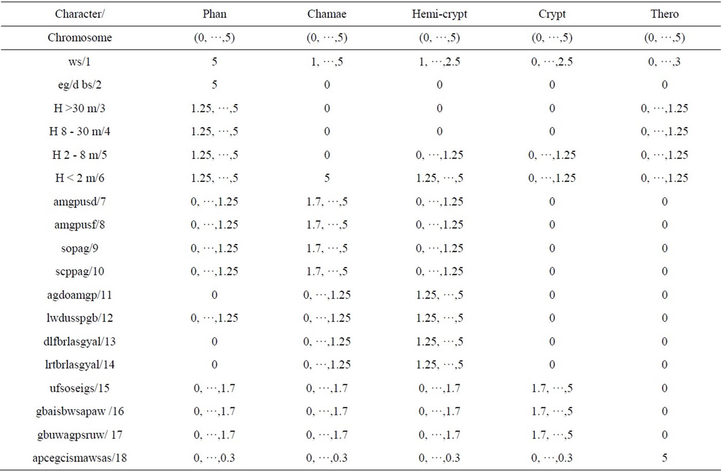
Table 3. Solutions and ranges for plant life form chromosomes.
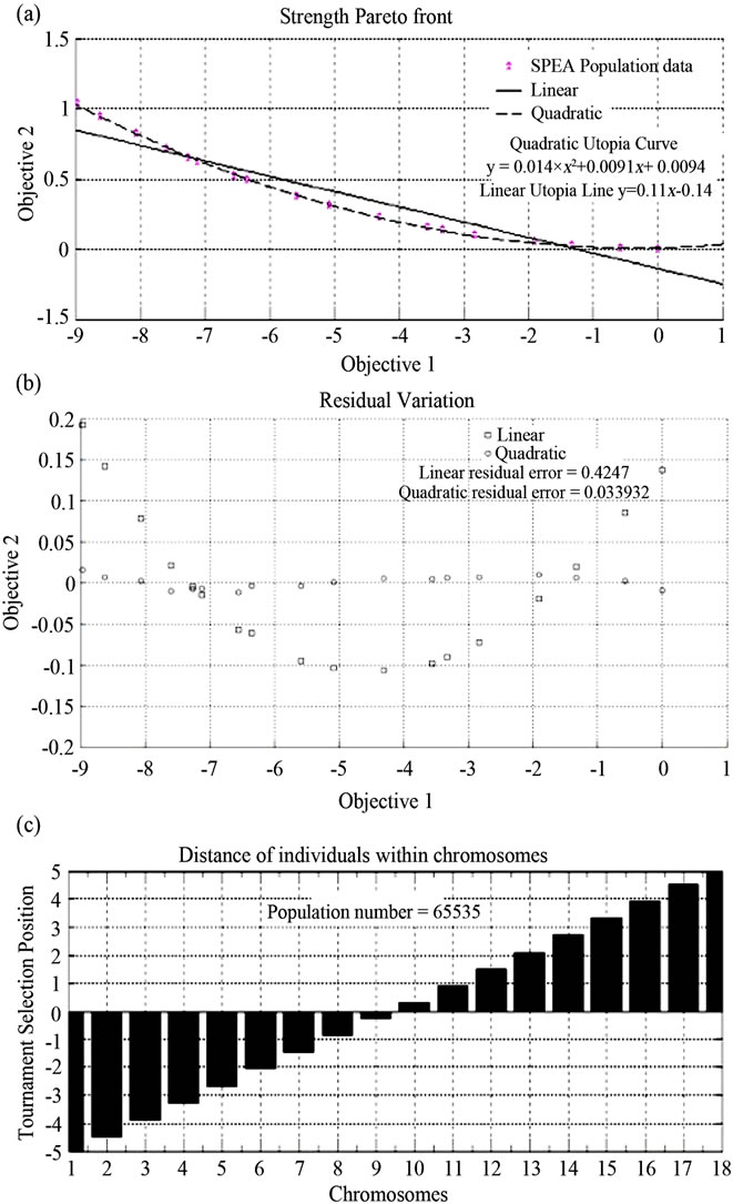
Figure 6. (a) Objective dispersal of the Strength Pareto Evolutionary population obtained for Ecuador; (b) Error of linear Utopia line and quadratic curve; (c) Illustration of how selection within the chromosome populations took place.
tions Ecuador and Macedonia as the strength Pareto shown in the previous section indicates. It is therefore possible to generate values of the Z plane with use of a surrogate Gaussian function model [14]. Rastrigin’s function is one such process function, which can be made use of in order to extrapolate values of a multimodal optimization.
Values of objective 1 (temperature) and objective 2 (precipitation) are extrapolated to the scale 0 - 5 and hence local minima of life-form percentage in Figure 7

Figure 7. Rastrigin’s function approximating distribution of plant life-forms within the Z hyperplane.
indicate the presence of the least present life-form (therophytes and hemi-cryptophytes in the case of Macedonia) and the maxima (peaks) of life-form percentage indicate the predominant life-form (in the case of Ecuador, phanerophytes). Use of the function is an effective method of extrapolating values in the Z hyperplane, given that the number of individual occurrences represents n in Equation (9). The 3 dimensional surface of the function is an appropriate surrogate illustrating how the characters of each life-form sub category overlap with one another in the spectrum of life-forms present in different ecosystems and locations. This point is discussed in the following section.
4. Discussion
In this paper we have presented a T-S-K logic based structure for the ordering of plant life-forms, carried out genetic programming of the life-forms and developed a method by which one can form functional approximation algorithms to elucidate distribution of elements within the Z utopia hyperplane.
The crucial difference between the use of Boolean mathematics to describe systems and the higher mathematic logic based methods employed is that the latter is devoid of semantic definition, establishing certainty in a previously distorted view [41, ch. 5], [42, ch. 4], [43, ch. 1]. In order to visualize the distribution of elements within a stochastic population we used a Gaussian process model, from which enhanced detail of the Z matrix can be extrapolated.
We implemented an efficient, minimized algorithmic approach using key elements of the water-energy dynamic for 2 candidate areas. We distributed a spectrum of life-forms, within given environments ideal for plant growth and comparatively more extreme conditions [3, 27]. Creation of the closed loop system for the areas covered allowed bounds of life-form spectrum distributions to be perceived as a continuum and primary nodes of life-forms identified, of which Ecuador is the most diverse and Macedonia is less diverse.
Further use of optimization methods enabled dispersal of the primary nodal number to give the secondary nodal number of life-forms. The distribution of the sub-categories of life-forms is of a binomial, poisson nature in agreement with previous climatic studies [15]. The distribution is summarized using linear and quadratic rules.
Using the multi-modal Rastrigin’s function showed that each dispersed life-form is expressed continuously for each individual life-form element, with zero mean and 0 - 1 variance (of the Z plane) within alternate environments. This method may be used to estimate proportions of individual species occurrences according to lifeform [28].
We propose the additional use of alternate functions (e.g. Sphere function, Schwefel’s function, Rosenbrock’s function) in order to indicate the functional approximation of all characters of plant species individual occurrence, either involving a simulative base, field data or an integration of the two (as in this paper). Using this method further unveils the dimensions of multi-objective orientated characters such as those of plant metabolites. Substantiation of the methods and patterns of this paper are useful not only to explore mathematical relations (niches and functional traits) but also to reinforce the requirement for enhanced protection of the areas covered by this study. Additionally modelling of climatic variables and the characters of plants modeled therein is enhanced in terms of accuracy and pattern distribution. Examples of the potential uses of this work include the finer scale structuring of phylogenetic trees, the patterning of prey-taxis relations [44-46], and measurement of quantitative trait loci such as those involved in biochemical pathways [47, ch. 8], [48]. Further, the informative value of the Z matrix is enhanced and expanding/contracting relational values may be explored [13,49]. Accessibility of mathematic methods to plant science and biogeography is facilitated. This is an important element to emphasize, especially with regard to vulnerable locations and indigenous populations in Ecuador, which are under threat of development [50]. Identification and expression of elements within priority conservation areas under threat of destructive human activity is of increasing importance, given the nature of the activities and the immediate effect on the concentrated biodiversity. There are thought to be more than two distinct niche processes operating in convergence and divergence of plant strategies [27,51]. It has been proven that strategy differentiation in plant species contributes to the maintenance of diversity in highly diverse locations. This work may assist with national policy formation in justification of direction of resources towards increased conservation and protection of vulnerable locations [52]. A starting place for implementation of conservation policy could manifest through local or national government partnerships with increased numbers of research based organizations, in order that the mathematical substantiation provided in this paper could be further investigated.
5. Acknowledgements
The authors would like to thank Prof. Kelly Swing for his encouragement and advice on policy implementation in preparation of this paper. This work was supported by financial contribution from the University of the West of England, UK.