Psychophysical Neuroeconomics of Decision Making: Nonlinear Time Perception Commonly Explains Anomalies in Temporal and Probability Discounting ()
1. Introduction
Canonical representations on Hermitian symmetric spaces  were introduced by Vershik-Gelfand-Graev [1] (for the Lobachevsky plane) and Berezin [2]. They are unitary with respect to some invariant non-local inner product (the Berezin form). Molchanov’s idea is that it is natural to consider canonical representations in a wider sense: to give up the condition of unitarity and let these representations act on sufficiently extensive spaces, in particular, on distributions. Moreover, the notion of canonical representation (in this wide sense) can be extended to other classes of semisimple symmetric spaces
 , in particular, to para-Hermitian symmetric spaces, see [3]. Moreover, sometimes it is natural to consider several spaces
  together, possibly with different
 , embedded as open
  -orbits into a compact manifold
 , where
  acts, so that
  is the closure of these orbits.
Canonical representations can be constructed as follows. Let  be a group containing
  (an overgroup),
  a series of representations of
  induced by characters of some parabolic subgroup
  associated with
  and acting on functions on
 . The canonical representations
  of
of  are restrictions of
  to
to .
.
In this talk we carry out this program for para-Hermitian symmetric spaces of rank one. These spaces are exhausted up to the covering by spaces  with
with ,
, . For these spaces
 , an overgroup is the direct product
  and canonical representations turn out to be tensor products of representations of maximal degenerate series and contragredient representations. These tensor products are studied in [4], see also [5]. So we lean essentially on these papers [4,5]. We decompose canonical representations into irreducible constituents and decompose boundary representations. Notice that in our case the inverse of the Berezin transform
  can be easily written: precisely it is the Berezin transform
 .
.
Canonical and boundary representations for  in the case
  (then
(then  is the hyperboloid of one sheet in
 ) were studied in [6]. For the two-sheeted hyperboloid in
 , it was done in [7].
In this paper we present only the main results. The detailed theory of canonical and boundary representations, for example, on a sphere with an action of the generalized Lorentz group, can be seen in [8].
Let us introduce some notation and agreements.
By  we denote
 . The sign
  denotes the congruence modulo 2.
For a character of the group  we shall use the following notation

where ,
,  ,
, .
.
For a manifold , let
, let  denote the Schwartz space of compactly supported infinitely differentiable
  -valued functions on
 , with a usual topology, and
  the space of distributions on
 —of anti-linear continuous functionals on
 .
.
2. The Space  and the Manifold
We consider the symmetric space  where
where ,
,  ,
, .
.
The group  acts on the space
  by
by
Let us write matrices in  in block form according to the partition
  of
of . Let us take the matrix

The subgroup  is just the stabilizer of this point
 , this subgroup consists of block diagonal matrices:

Thus, our space  is the
  -orbit of
 , it consists of matrices of rank one and trace one.
Equip  with the standard inner product
 , let
, let . Let
. Let  be the sphere
 . Let
. Let  be the Euclidean measure on
 . The group
  acts on
  by
by .
.
Let  be a cone in
  consisting of matrices
  of rank one. Therefore, the space
  is the section of
  by the hyperplane
 .
.
Introduce a norm  in
in  by
by

where the prime denotes matrix transposition.
Let  be the section of
  by
by .
.
Define a map  by
by

It is a two-fold covering. The measure  defines a measure
  on
on  by
by

The action of the group  on
on  gives the following action of
  on
on :
:
In particular, the subgroup , a maximal compact subgroup, acts on
  by translations:

Let us consider on  the function
 (1)
(1)
The action on  has three orbits: namely, two open orbits (of dimension
 ):
):  and
and  and one orbit of dimension
 :
:  . The orbit
  is a Stiefel manifold, it is the boundary of
 . Denote
 . Each of orbits
  can be identified with the space
 . The map is constructed by means of generating lines of the cone
 .
.
3. Maximal Degenerate Series Representations
Recall [4] maximal degenerate series representations ,
,  ,
,  , of the group
 . Let
. Let  be the subspace of
  consisting of functions
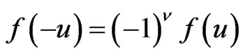
  of parity
 :
: . The representations
  act on
  by
by

4. Representations of  Associated with
Recall [5] a series of representations  of the group
  associated with the space
 .
.
Denote by  the space of functions
  in
in  of parity
 :
:

The representation  acts on
  by
by
 (2)
(2)
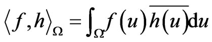
Let  denote the following sesqui-linear form
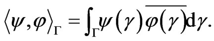 (3)
(3)
Define an operator  on
on  by
by

It intertwines  and
and . The operator
  is a meromorphic function of
 . Let us normalize this operator (multiplying it by a function of
 ) such that the normalized operator
  is an entire non-vanishing function of
 .
.
There are three series of unitarizable irreducible representations. The continuous series consists of  with
with ,
,  , the inner product is (3). The complementary series consists of
  with
with
 , the inner product is
with a factor. The discrete series consists of the representations  where
where ,
,
 ,
,  , which are factor representations of
 on the quotient spaces
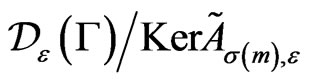 . The representations
  with the same
  and different
 are equivalent. It is convenient to take
  where
where  for odd
  and
and  for even
 . The inner product is induced by the form
 .
.
5. Canonical Representations
We define canonical representations ,
,  ,
,  , of the group
  as tensor products:

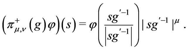
They can be realized on : let
: let  denote the subspace of
  consisting of functions
  of parity
 :
: , then the representation
  acts on
  by a formula similar to (2):

The inner product
 (4)
(4)
is invariant with respect to the pair , i.e.
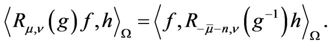 (5)
(5)
Consider an operator  on
on  defined by

It turns out that the composition  is equal to the identity operator
  up to a factor. We can take
  such that
namely,

With the form (4) the operator  interacts as follows:
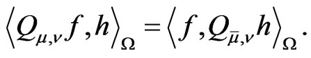 (6)
(6)
This operator  intertwines the representations
  and
and , i.e.

Let us call it the Berezin transform.
Let  be the space of distributions on
  of parity
 . We extend
  and
and  to
to  by (5) and (6) respectively and retain their names and the notation.
Let us introduce the following Hermitian form  on
on :
:

Let us call this form the Berezin form.
6. Boundary Representations
The canonical representation  gives rise to two representations
  and
and  associated with the boundary
  of the manifolds
  (boundary representations). The first one acts on distributions concentrated at
 , the second one acts on jets orthogonal to
 .
.
We can introduce “polar coordinates” on  corresponding to the foliation of
  into
into  -orbits. The
  - orbits are level surfaces of the function
 , see (1). For
  the
the  -orbits are diffeomorphic to
 . In these coordinates the measure
  on
on  is
is

where  is the measure on
 .
.
Let  be a function in
 . Consider it as a function of polar coordinates. Consider its Taylor series
  in powers of
 . Here
  are functions in
 . Denote by
 ,
,  ,
,  , the space of distributions in
 , having the form

where ,
,  is the Dirac delta function on the real line,
  its derivatives. Let
  .
.
Denote by  Taylor coefficients of the function
 . The distribution
  acts on a function
  as follows:
 (7)
(7)
Denote by  the restriction of
  to
to . This representation is written as a upper triangular matrix with the diagonal
 ,
, .
.
Distributions in  can be extended in a natural way to a space wider than
 . Namely, let
be the space of functions  of class
  on
on  and
and  of parity
  and having the Taylor decomposition of order
 :
:

where . Then (7) keeps for
  with
with .
.
Let  denote the column of Taylor coefficients
 . The representation
  acts on these columns:

It is written as a lower triangular matrix with the diagonal ,
, .
.
The boundary representations  and
and  are in a duality.
7. Poisson and Fourier Transforms
Let us write operators  and
and  intertwining representations
  and
and . We call them Poisson and Fourier transforms associated with canonical representations.
The Poisson transform  is a map
  given by

It intertwines  with
with . Here we consider
 as the restriction to
  of the representation
  acting on distributions in
 .
.
For a  -finite function
  and
and  the Poisson transform has the following decomposition in powers of
 :
:

where  has polar coordinates
 . Here
  and
and
 are certain operators acting on
 . The factors
  and
and  give poles of the Poisson transform in
  depending on
 :
:
 (8)
(8)
where  and
and ,
, . If a pole belongs only to one of series (8), then the pole is simple, and if a pole belongs to both series (8), then
  and the pole is of the second or first order.
Let the pole ,
,  , be simple. The residue
  of
of  at this pole is an operator
 . Denote the image of this operator by
 .
.
The Fourier transform  is a map
  given by

It intertwines  with
with .
.
The Fourier and Poisson transforms are conjugate to each other:

Poles in  of the Fourier transform are situated at points
 (9)
(9)
where  and
and ,
, . If a pole belongs only to one of the series (9), then the pole is simple, and if a pole belongs to both series (9), then
  and the pole is of the second or first order.
Let the pole ,
,  , be simple.
The residue  of
of  at this pole is a “boundary” operator
 ,
, . The operator
  is defined in terms of Taylor coefficients
 : it is a linear combination of functions
 . Therefore, we may consider the following operator
  acting on columns
 of functions
 : this operator to any column
  assigns the column
 of functions in the same space
 —by the same formulas without
 . This operator
  is given by a lower triangular matrix.
8. Decomposition of Boundary Representations
The meromorphic structure of the Poisson and Fourier transforms is a basis for decompositions of boundary representations  and
and .
.
Let the pole  of the Poisson transform is simple, in particular, it happens when
 . Then the boundary representation
  is diagonalizable which means that
  decomposes into the direct sum of
 , and the restriction of
to  is equivalent to
  (by means of
 ).
).
If a pole is of the second order, then the decomposition of  contains a finite number of Jordan blocks, this number depends on
 .
.
Let the pole  of the Fourier transform is simple, in particular, when
 . Then the matrix
  is diagonalizable which means that
 is a diagonal matrix. Its diagonal is
 ,
, .
.
If a pole is of the second order, then the decomposition of  contains a finite number of Jordan blocks, this number depends on
 .
.
9. Decomposition of Canonical Representations
Let us write decomposition of canonical representations. We restrict ourselves to a generic case:  lies in strips

Case (A): .
.
Theorem 1 Let . Then the canonical representation
  decomposes—as the quasiregular representation [5]—into irreducible unitary representations of continuous and discrete series with multiplicity one. Namely, let us assign to a function
  the family of its Fourier components
 ,
,  ,
,  ,
,  , and
, and
 ,
, . This correspondence is
  equivariant. There is an inversion formula:
 (10)
(10)
and a “Plancherel formula” for the Berezin form:
 (11)
(11)
Here  and
and  stand for the Plancherel measure for
 , see [5], the factor
  is given by following formula:

Case (B): .
.
Here we continue decomposition (10) analytically in  from
from  to
to ,
, . Some poles in
  of the integrand intersect the integrating line—the line
 . They are poles
  and
and 
 of the Poisson transform with
 . They give additional summands to the right hand side. So after the continuation we obtain:
 (12)
(12)
where the integral and the series mean the same as in (10) and

 are some numbers.
Similarly, the continuation of (11) gives
 (13)
(13)
where the integral and the series mean the same as in (11) and  are some numbers.
The operators ,
,  , can be extended from
 to the space
  and therefore to the sum

Then these operators  turn out to be projection operators onto
 . Moreover, there are some “orthogonality relations” for them. Decomposition (13) can also be extended to the space
 . This decomposition is a “Pythagorean theorem” for decomposition (12).
Theorem 2 Let ,
, . Then the space
  has to be completed to
 . On this space the representation
  splits into the sum of two terms: the first one decomposes as
  does in Case (A), the second one decomposes into the sum of
  irreducible representations
 ,
, . Namely, let us assign to any
  the family

where ,
,  ,
, . This correspondence is
  -equivariant. There is an inverse formula, see (12), and a “Plancherel formula”, see (13).
Case (C): .
.
Now we continue decomposition (10) analytically in  from
from  to
to . Here poles
  and
and ,
,  ,
,  , of the integrand (they are poles of the Fourier transform) give additional terms. We obtain
 (14)
(14)
where the integral and the series mean the same as in (10) and

 some numbers. The operators
  can be extended to the space
 ,
, . Denote by
  the image of
 . It turns out that the operators
  are projection operators onto
  and for them there are some “orthogonality relations”.
Now we continue decomposition (11) from  to
to . Poles of the integrand which intersect the integrating line
  and give additional terms (they are poles of both Fourier transforms) turn out fortunately to be of the first order, since at these points the function
  as a function of
  has zero of the first order. After the continuation we obtain:
 (15)
(15)
where the integral and the series mean the same as in (11),  some numbers. It is a “Pythagorean theorem” for decomposition (14).
Theorem 3 Let ,
, . Then the representation
  considered on the space
  splits into the sum of two terms. The first one acts on the subspace of functions
  such that their Taylor coefficients
  are equal to 0 for
  and decomposes as
  does in Case (A), the second one decomposes into the direct sum of
  irreducible representations
 ,
,  acting on the sum of the spaces
 . There is an inversion formula, see (14), and a “Plancherel formula” for the Berezin form, see (15).