Relationship between Maximum Principle and Dynamic Programming in Stochastic Differential Games and Applications ()
1. Introduction
Game theory has been an active area of research and a useful tool in many applications, particularly in biology and economic. Among others, there are two main approaches to study differential game problems. One approach is Bellman’s dynamic programming, which relates the saddle points or Nash equilibrium points to some partial differential Equations (PDEs) which are known as the Hamilton-Jacobi-Bellman-Isaacs (HJBI) Equations (see Elliott [1], Fleming and Souganidis [2], Buckdahn et al. [3], Mataramvura and Oksendal [4]). The other approach is Pontryagin’s maximum principle, which finds solutions to the differential games via some Hamiltonian function and adjoint processes (see Tang and Li [5], An and Oksendal [6]).
Hence, a natural question arises: Are there any relations between these two methods? For stochastic control problems, such a topic has been discussed by many authors (see Bensoussan [7], Zhou [8], Yong and Zhou [9], Framstad et al. [10], Shi and Wu [11], Donnelly [12], etc.) However, to the best of our knowledge, the study on the relationship between maximum principle and dynamic programming for stochastic differential games is quite lacking in literature.
In this paper, we consider one kind of zero-sum stochastic differential game problem within the frame work of Mataramvura and Oksendal [4] and An and Oksendal [6]. However, we don’t consider jumps. This more general case will appear in our forthcoming paper. For our problem in this paper, [4] related its saddle point to some HJBI Equation and obtained the stochastic verification theorem. [6] proves both sufficient and necessary maximum principles, which state some conditions of optimality via the Hamiltonian function and adjoint Equation. The main contribution of this paper is that we connect the maximum principle of [6] with the dynamic programming of [4], and obtain relations among the adjoint processes, the generalized Hamiltonian function and the value function under the assumption that the value function is enough smooth. As applications, we discuss a portfolio optimization problem under model uncertainty in the financial market. In this problem, the optimal portfolio strategies for the trader (representative agent) and the “worst case scenarios” (see Peskir and Shorish [13], Korn and Menkens [14]) for the market, derived from both maximum principle and dynamic programming approaches independently, coincide. The relation that we obtained in our main result is illustrated.
The rest of this paper is organized as follows. In Section 2, we state our zero-sum stochastic differential game problem. Under suitable assumptions, we reformulate the sufficient maximum principle of [6] by adjoint Equation and Hamiltonian function, and the stochastic verification theorem [4] by HJBI Equation. In Section 3, we prove the relationship between maximum principle and dynamic programming for our zero-sum stochastic differential game problem, under the assumption that the value function is enough smooth. A portfolio optimization problem under model uncertainty in the financial market is discussed in Section 4, to show the applications of our result.
Notations: throughout this paper, we denote by  the space of n-dimensional Euclidean space, by
  the space of
  matrices, by
  the space of
  symmetric matrices.
  and |.| denote the scalar product and norm in the Euclidean space, respectively.
  appearing in the superscripts denotes the transpose of a matrix.
2. Problem Statement and Preliminaries
Let  be given, suppose that the dynamics of a stochastic system is described by a stochastic differential Equation (SDE) on a complete probability space
  of the form
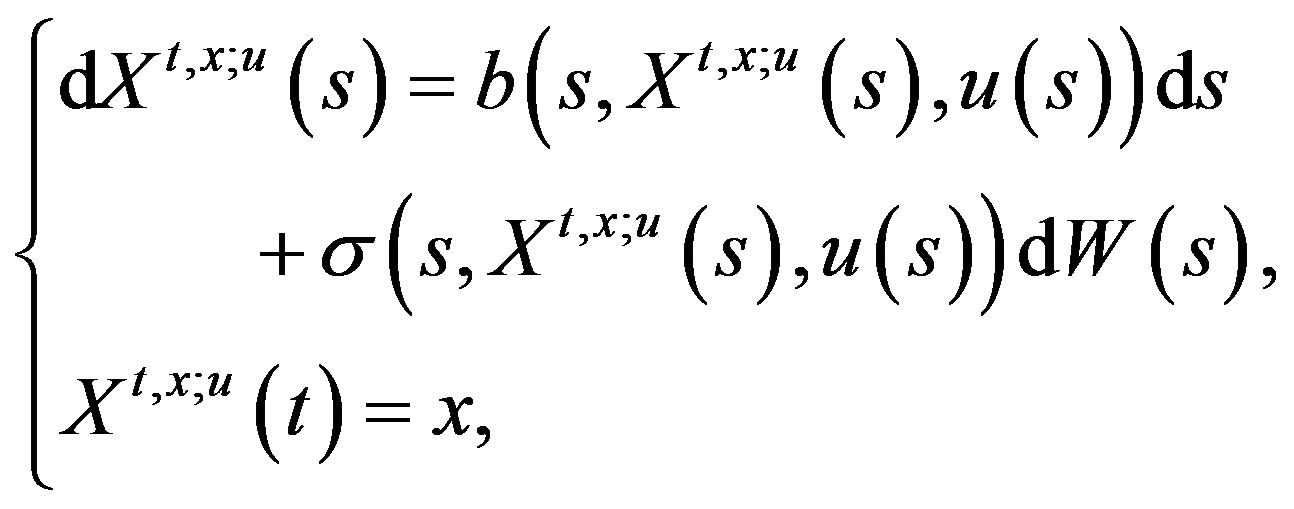 (1)
(1)
with initial time  and initial state
 . Here
  is a d-dimensional standard Brownian motion. For given
 , we suppose the filtration
  is generated as the following
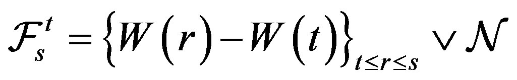 ,
,
where  contains all P-null sets in
  and
and  denotes the
  -field generated by
 . In particular, if the initial time
 , we write
 .
.
In the above,
 ,
,

are given continuous functions, where  is nonempty and convex. The U-valued process
 is the control process.
For any , we denote by
  the set of
  -adapted processes. For given
and , an
, an  -valued process
  is called a solution to (1) if it is an
  -adapted process such that (1) holds. We refer to such
  as an admissible control and
  as an admissible pair.
We make the following assumption.
(H1) There exists a constant  such that for all
 , we have
 ,
,
 ,
,
 .
.
For any , under (H1), it is obvious that SDE (1) has a unique solution
 .
.
Let  and
and  be continuous functions. For any
  and admissible control
 , we define the following performance functional
 (2)
(2)
Now suppose that the control process has the form
 , (3)
, (3)
where  and
and  are valued in two sets
  and
and , respectively. We let
  and
and  be given families of admissible controls
  and
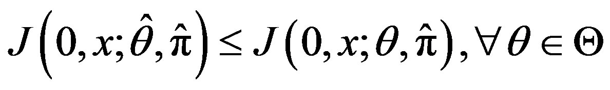
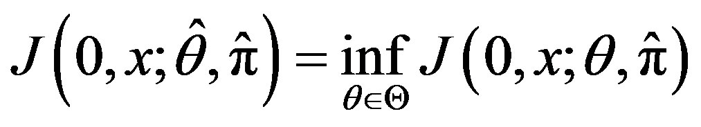
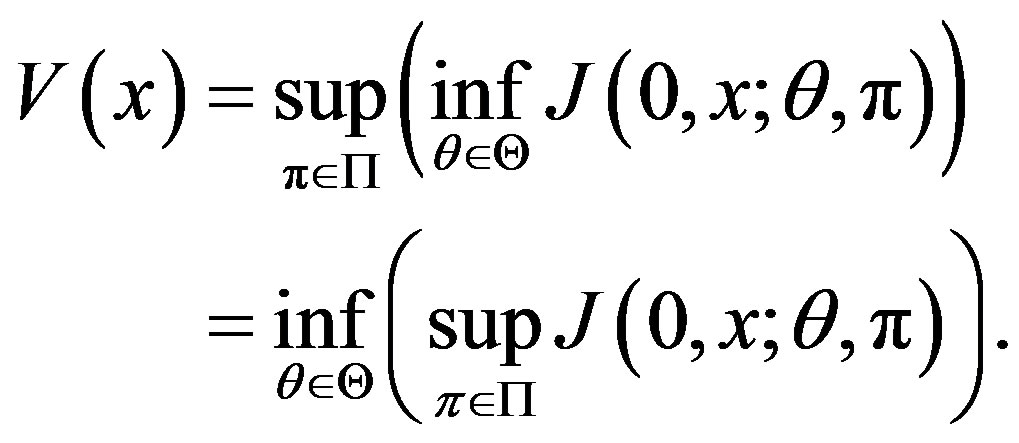
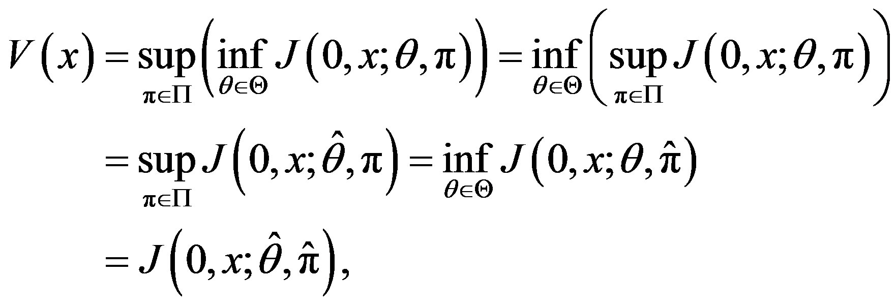
and , respectively. The zero-sum stochastic differential game problem is to find
  such that
 (4)
(4)
for given , with
 .
.
Such a control process (pair)  is called an optimal control or a saddle point of our zero-sum stochastic differential game problem (if it exists). And the corresponding solution
  to (1) is called the optimal state.
The intuitive idea is that there are two players, I and II. Player I controls  and Player II controls
 . The actions of the two players are antagonistic, which means that between Players I and II there is a payoff
  which is a cost for player I and a reward for Player II.
We now define the Hamiltonian function

by
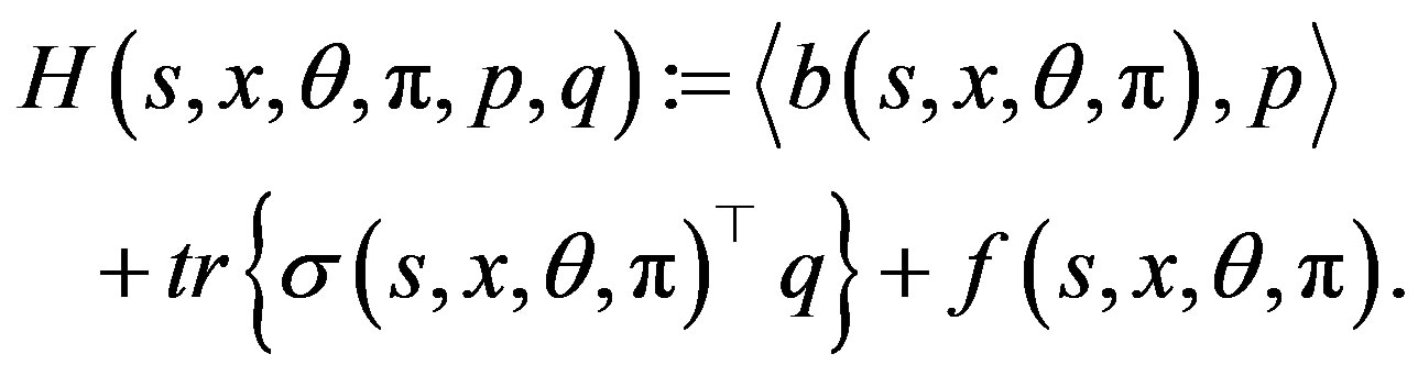 (5)
(5)
In addition, we need the following assumption.
(H2) B, σ, f are continuously differentiable in  and
and  is continuously differentiable in
 . Moreover,
  are bounded and there exists a constant
  such that for all
 , we have

The adjoint Equation in the unknown  -adapted processes
  is the backward stochastic differential Equation (BSDE) of the form
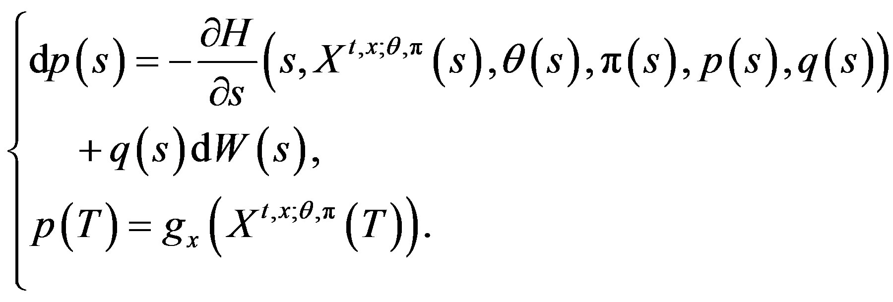 (6)
(6)
For any , under (H2), we know that BSDE (6) admits a unique
  -adapted solution
 .
.
We now can state the following sufficient maximum principle which is Corollary 2.1 in An and Oksendal [6].
Lemma 2.1 Let (H1), (H2) hold and  be fixed. Suppose that

with corresponding state process .
.
Let  and
and  be
be  and
and
 , respectively. Suppose that there exists a solution
  to the corresponding adjoint Equation (6). Moreover, suppose that for all
 , the following minimum/maximum conditions hold:
 (7)
(7)
1) Suppose that for all  is concave and

is concave. Then
 and
and
 .
.
2) Suppose that for all  is convex and

is convex. Then
 and
and
 .
.
3) If both Cases (1) and (2) hold (which implies, in particular, that g is an affine function), then

is an optimal control (saddle point) and
 (8)
(8)
Next, when the control process  is Markovian, then we can define the generator
  of diffusion system (1) by
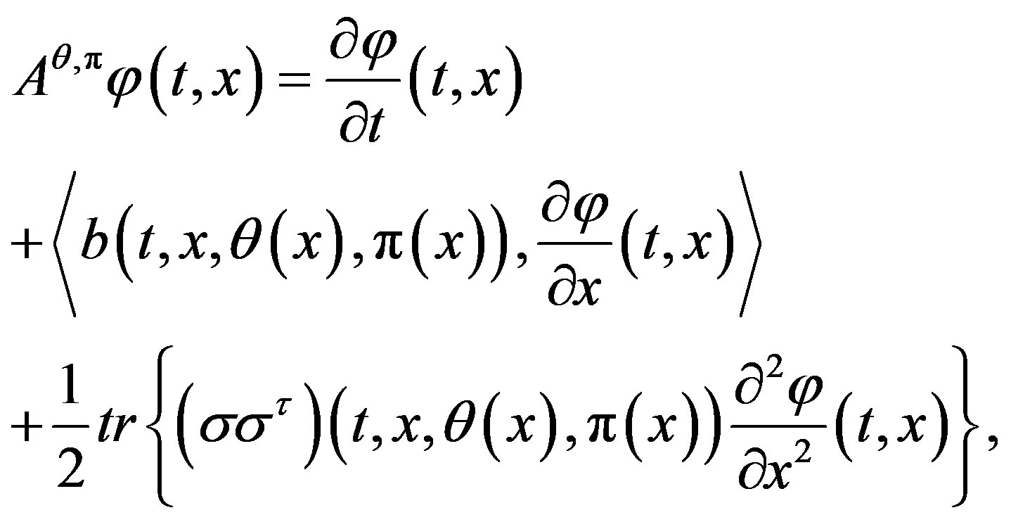 (9)
(9)
where .
.
The following result is a stochastic verification theorem of optimality, which is an immediate corollary of Theorem 3.2 in Mataramvura and Oksendal [4].
Lemma 2.2 Let (H1), (H2) hold and  be fixed. Suppose that there exists a

and a Markovian control process  such that 1)
2) 
3) 
4) ,
,
 5) the family
 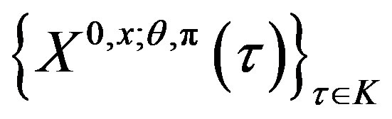 is uniformly integrable for all
 ,
, , where
  is the set of stopping times
 . (10)
Then
 (11)
(11)
and  is an optimal Markovian control.
3. Main Result
In this section, we investigate the relationship between maximum principle and dynamic programming for our zero-sum stochastic differential game problem. The main contribution is that we find the connection between the value function , the adjoint processes
  and the following generalized Hamiltonian function

defined by
 (12)
(12)
Our main result is the following.
Theorem 3.1 Let (H1), (H2) hold and 
be fixed. Suppose that  is an optimal Markovian control, and
  is the corresponding optimal state. Suppose that the value function
 then
then
(1)
 (13)
(13)

(2)
 (14)
(14)
 and
and
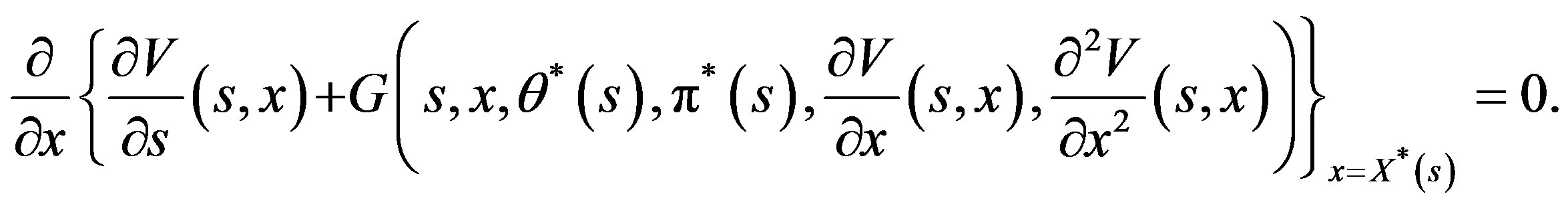
(3)
 (15)
(15)

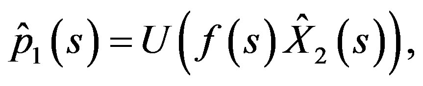
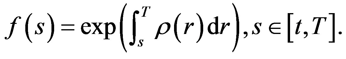
Further, suppose that

and  is also continuous. For any
 , define
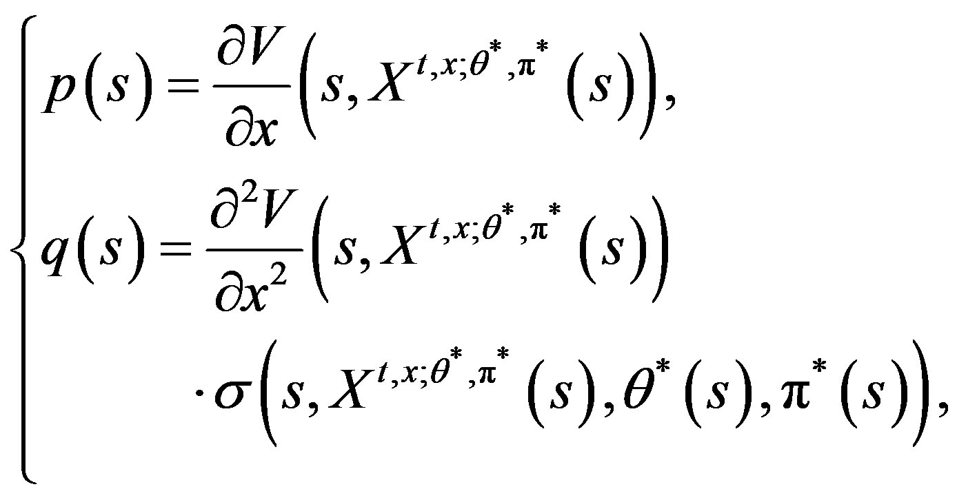 (16)
(16)
then  solves the adjoint Equation (6).
Proof. (13), (15) can be obtained from the HJBI Equation (10), by the definitions of the generator  in (9) and the generalized Hamiltonian function
  in (12).
We proceed to prove the second part. If

and  is also continuous, then from (15), we have
This is equivalent to

where

with 
On the other hand, applying Ito’s formula to , we get

Note that
 .
.
Hence, by the uniqueness of the solutions to (6), we obtain (16). The proof is complete.□
4. Applications
In this section, we will discuss a portfolio optimization problem under model uncertainty in the financial market, where the problem is put into the framework of a zero-sum stochastic differential game. The optimal portfolio strategies for the investor and the “worst case scenarios” for the market, derived both from maximum principle and dynamic programming approaches independently, coincide. The relation that we obtained in our main result Theorem 3.1 is illustrated.
Suppose that the investors have two kinds of securities in the market for possible investment choice:
(1) a risk-free security (e.g. a bond), where the price  at time
  is given by

here  is a deterministic function;
(2) a risky security (e.g. a stock), where the price  at time
  is given by

here  is a one-dimensional Brownian motion and
  are deterministic functions with
 .
.
Let  be a portfolio for the investors in the market, which is the proportion of the wealth invested in the risky security at time
 .
.
Given the initial wealth , we assume that
  is self-financing, which means that the corresponding wealth process
  admits the following dynamics
 (17)
(17)
A portfolio  is admissible if it is an
  -adapted process and satisfies

The family of admissible portfolios is denoted by .
.
Now, we introduce a family  of measures
  parameterized by processes
  such that
 (18)
(18)
where
 (19)
(19)
We assume that
 (20)
(20)
If  satisfies
 (21)
(21)
then  is a probability measure. If in addition,
 (22)
(22)
then

is an equivalent local martingale measure. But here we do not assume that (22) holds.
All  satisfying (20) and (21) are called admissible controls of the market. The family of admissible controls
  is denoted by
 .
.
The problem is to find  such that
 (23)
(23)
where  is a given utility function, which is increasing, concave and twice continuously differentiable on
 .
.
We can consider this problem as a zero-sum stochastic differential game between the agent and the market. The agent wants to maximize his/her expected discounted utility over all portfolios  and the market wants to minimize the maximal expected utility of the agent over all “scenarios”, represented by all probability measures
 .
.
To put the problem in a Markovian framework so that we can apply the dynamic programming, define
 (24)
(24)
where  denote the initial time of the investmentand
 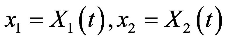 are the initial values of the process
  given by
 (25)
(25)
which is a 2-dimensional process combined the Radon-Nikodym process  with the wealth process
 .
.
4.1. Maximum Principle Approach
To solve our problem by maximum principle approach, that is, applying Lemma 2.1, we write down the Hamiltonian function (5) as
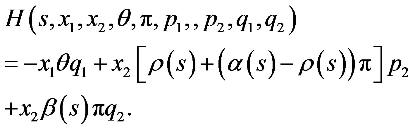 (26)
(26)
The adjoint Equations (6) are
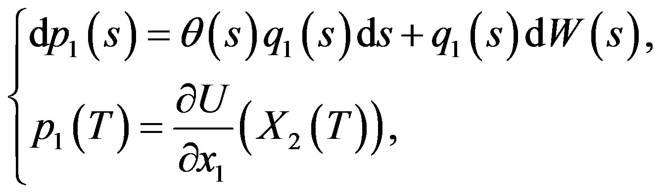 (27)
(27)
and
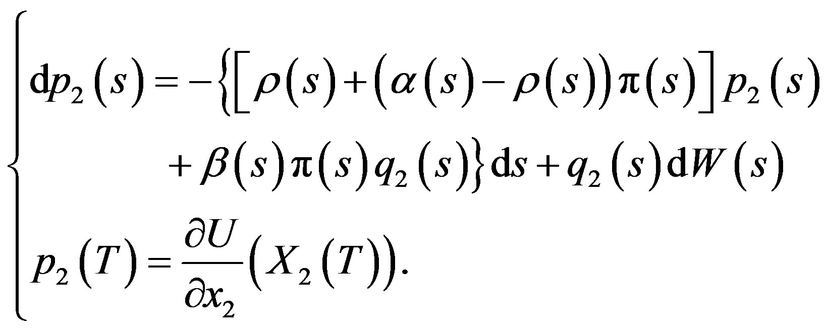 (28)
(28)
Let  be a candidate optimal control (saddle point) and let
  be the corresponding state process, with corresponding solution

to the adjoint Equations.
By (7) in Lemma 2.1, we first maximize the Hamiltonian function  over all
 . This gives the following condition for a maximum point
 :
:
 (29)
(29)
Then, we minimize  over all
 , and get the Following condition for a minimum point
 :
:
 (30)
(30)
We try a process  of the form
 (31)
(31)
with a deterministic differential function .
.
Differentiating (31) and using (17), we get
 (32)
(32)
Comparing this with the adjoint Equation (27) by equating the  coefficients respectively, we get
 (33)
(33)
and
 (34)
(34)
Substituting (33) into (30), we have
 (35)
(35)
or
 (36)
(36)
Now, we try a process  of the form
 (37)
(37)
Differentiating (37) and using (17), (36), we get
 (38)
(38)
Comparing this with the adjoint Equation (28), we have
 (39)
(39)
and
 (40)
(40)
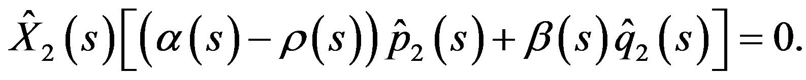
Substituting (39) into (29), we have

or
 (41)
(41)
From (40), we get

or
 (42)
(42)
i.e.,
 (43)
(43)
Let , we have proved the following theorem.
Theorem 4.1 The optimal portfolio strategy  for the agent is
 (44)
(44)
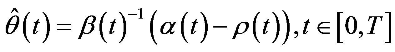
The optimal “scenario”, that is, the optimal probability measure for the market is to choose  such that
 (45)
(45)
That is, the market minimize the maximal expected utility of the agent by choosing a scenario (represented by a probability law ), which is an equivalent martingale measure for the market (see (22)).
In this case, the optimal portfolio strategy for the agent is to place all the money in the risk-free security, i.e., to choose  for all
 .
.
This result is the counterpart of Theorem 4.1 in An and Oksendal [6] without jumps with complete information.
4.2. Dynamic Programming Approach
To solve our problem by dynamic programming approach, that is, applying Lemma 2.2, we write down the generator  of the diffusion system (25) as
 (46)
(46)
for .
.
Applying to our setting, the HJBI Equation (10) gets the following form
 (47)
(47)
We try a  of the form
 (48)
(48)
for some deterministic function  with
with . Note that conditions (i), (ii), (iii) in (47) can be rewritten as
 (49)
(49)
 (50)
(50)
Maximizing  over all
  gives the following first-order condition for a maximum point
 :
:
 (51)
(51)
We then minimize  over all
  and get the following first-order condition for a minimum point
 :
:
 (52)
(52)
From (52) we conclude that
 (53)
(53)
which substituted into (51) gives
 (54)
(54)
And the HJBI Equation (iii)  states that with these values of
  and
and , we should have

or
 (55)
(55)
i.e.,
 (56)
(56)
We have proved the following result.
Theorem 4.2 The optimal portfolio strategy  for the agent is
 (57)
(57)
(i.e., to put all the wealth in the risk-free security) and the optimal “scenario” for the market is to choose  such that
 (58)
(58)
(i.e., the market chooses an equivalent martingale measure or risk-free measure  for the market).
This result is the counterpart of Theorem 2.2 in Oksendal and Sulem [15] without jumps.
4.3. Relationship between Maximum Principle and Dynamic Programming
We now verify the relationships in Theorem 3.1. In fact, relationship (13), (14), (15) is obvious from (47). We only need to verify the following relations

and

Note that , the above relations are easily obtained from (48), (31), (37), (33) and (39).
5. Conclusions and Future Works
In this paper, we have discussed the relationship between maximum principle and dynamic programming in zerosum stochastic differential games. Under the assumption that the value function is smooth, relations among the adjoint processes, the generalized Hamiltonian function and the value function are given. A portfolio optimization problem under model uncertainty in the financial market is discussed to show the applications of our result.
Many interesting and challenging problems remain open. For example, what is the relationship between maximum principle and dynamic programming for stochastic differential games without the illusory assumption that the value function is smooth? This problem may be solved in the framework of viscosity solution theory (Yong and Zhou [9]). Another topic is that we can continue to investigate the relationship between maximum principle and dynamic programming for forward and backward stochastic differential games, and then study its applications to stochastic recursive utility optimization problem under model uncertainty (Oksendal and Sulem [16]). Such topics will be studied in our future work.
6. Acknowledgements
This work is supported by National Natural Science Foundations of China (Grant No. 11301011 and 11201264) and Shandong Province (ZR2011AQ012).