Wavelet Interpolation Method for Solving Singular Integral Equations ()
1. Introduction
In the early 1900s, Ivar Fredholm solved the integral equations named after him,

where the function  and continuous kernel
  are given, and the unknown function y(x) is to be determined. A numerical method of solving this equation has been shown in [1]. In this study, we discuss the numerical solution of singular Fredholm integral equation of the second kind which is defined as follows:
 (1)
(1)
where the functions  and
and  are given, the numerical solution for Equation (1) is to provide an approximation for the unknown function
 . In fact, Equation (1) is known as an Abel’s integral equation which is defined by Niels Henrik Abel. There are many approaches to find a numerical solution of the Abel’s equation [2], such as Gauss-Jacobi quadrature rule which was proposed by Fettis (1964), orthogonal polynomials expansion by Kosarev (1973), the Chebyshev polynomials of the first kind by Piessens and Verbaeten (1973) and Piessens (2000), etc. Recently, K. Maleknejad, M. Nosrati and E. Najafi solved the equation by using wavelet Galerkin method [3]. Here we used Coiflets to find a numerical solution of Equation (1).
The Coiflets are discussed in the next section briefly. In Section 3, we solve Abel’s Equation (1) by using Coiflets. The error analysis is discussed in Section 4. Finally, we apply our method for two singular equations in the examples and compare our method with other method [3]. We obtain numerical solutions which have achieved better accuracy.
2. Coiflets and Wavelet Interpolation
In the context of wavelet theory, we usually deal with wavelets and scaling functions [4]. The wavelet function is defined by building a sequence upon scaling functions generated by . Choosing some suitable sequence,
  , we obtain the following dilation equation,
A nested of subspaces  of
of  is defined such that,

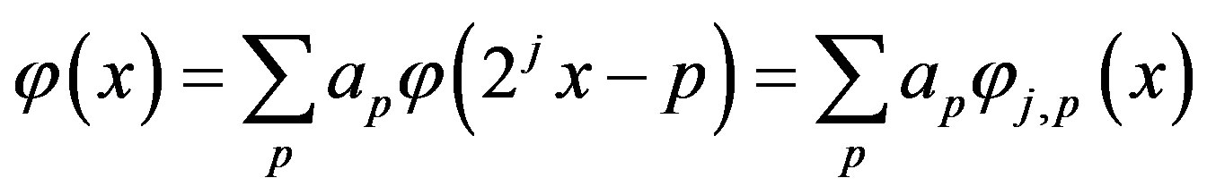
which means that for any function  it can be expressed as:

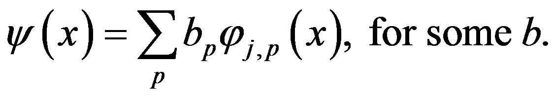
If the basis functions of a subspace are orthogonal at the same level, then a given function  can be expressed as follows:
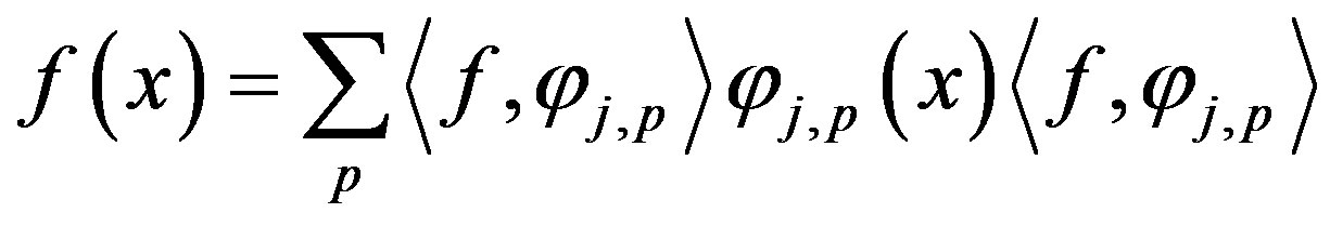
where

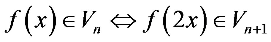
If the nested sequence of the subspaces  has the following properties then it is called a multiresolution analysis (MRA):
1) 
2) 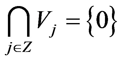
3) 
4) 
5) there exists a function  such that
 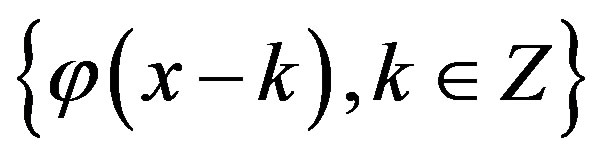 is an orthogonal basis for
 .
.
The wavelet function is constructed in the orthogonal complement of each subspace  in
in  which is denoted by
 . This means
 . Since

we have  and
and . The set
  forms a basis for
 , and can be obtained from the following equation:
The orthogonally of  on
on  means that any member of
  is orthogonal to the members of
 , that is,

In fact, scaling function and wavelet have the following properties:
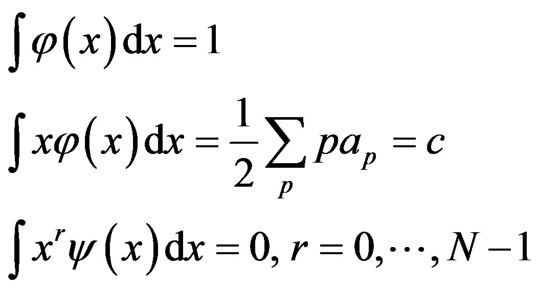
where  is the compact support of
  and
and 
In what follows, we will recall a scaling function interpolation theorem and the definition of Coiflets. As an application, we will use Coiflets and this interpolation formula to find numerical solutions of singular integral equations.
Definition 2.1. The Coifman wavelet system (Coiflet) of order L is an orthogonal multiresolution wavelet system with


Lin and Zhou proved the following interpolation theorem in R2 and :
:
Theorem 2.1. [5] Assume the function , where
  is a bounded open set in
 ,
,  Let, for
 ,
,

where the index

and sup denotes the support of the function.
In addition the moments  satisfy

Then
 (2)
(2)
where  is a constant depending only on
  and diameter of
 ;
;

3. Solving Singular Fredholm Integral Equation Using Coiflets
This section provides a method of finding numerical solution of Equation (1). In what follows, we assume that  and
and  satisfies Lipschitz condition. The unknown function
  in Equation (1) can be expressed in term of scaling functions in the subspacev, where the function
  is approximated by
  such that;
 (3)
(3)
To find the numerical solution we need to determinate the unknowns  in Equation (3).
By substituting Equation (3) in (1) we have the following equation,

which is equivalent to the equation,
 (4)
(4)
By providing sufficient collocation points in  for Equation (4) we will have a linear system of linear equations with unknown
 . In fact, the linear system can be written as the following matrix equation,

where ,
,
 and
and

is obtained from the left hand side of Equation (4). Subsequently, we substitute the solutions of ap into Equation (3), and obtain an approximate solution of the integral equation.
4. Error Analysis
The integral Equation (1) can be rewritten as follows [3].
 (5)
(5)
where

Then the integral Equation (1) is equivalent to the following equation,
 (6)
(6)
The next theorem shows the convergence rate of our method for solving Equation (1). Without loss of generality, we suppose that the integral equation is defined on the interval .
.
Theorem 4.1. In Equation (1), suppose that the function k satisfies the Lipchitz condition. Moreover,  is continuous on the interval
 . For
. For ,
,
 (7)
(7)
is an approximate solution of the unknown function in Equation (1) with coefficients obtained in Section 3. Then

for some constant c.
Proof: We prove in two cases, one at singularities (case 1) and the other at the points  (case 2).
Case 1. In Equation (1) when , the function
  satisfies the Lipchitz condition and the function
  is continuous, then Equation (1) is equivalent to Equation (6), then the function
  which gives us the exact solution.
Case 2. In this case we don’t have singularities, and Equation (1) is equivalent to Equation (6) and  . Subtracting Equation (7) from (6) and applying the norm, we have
 (8)
(8)
The unknown function  can be interpolated using Coiflet such that
 (9)
(9)
If we add and subtract Equation (9) to (8), then Equation (8) becomes:
 (10)
(10)
Notice that  is finite, then let
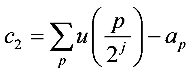
and by using Equation (2),

Equation (10) becomes

for some constant c which is absorbed from the above inequality.
5. Numerical Examples
In the following examples we are solving singular Fredholm integral equation of the second kind by using Coiflet of order 5 and calculate errors between the exact and numerical solutions at level j = −10. The errors are shown in Table 1.
Example 1.
We solve the singular integral equation

Table 1. The absolute error for Examples 1 and 2.

with

and the exact solution is .
.
Example 2.
We consider the following singular integral equation

with the exact solution .
.
6. Conclusion
We apply our method to the same examples shown in [3]. Table 1 indicates that our solutions have better accuracy than the solutions obtained in [3]. Our method is robust and efficient. There are other questions such as finding solutions at different levels of subspaces and solving nonlinear integral equations which will be our next research projects.