Some Additional Moment Conditions for a Dynamic Count Panel Data Model with Predetermined Explanatory Variables ()
1. Introduction
Since the pioneering works conducted by [4,5], which aim at estimating the knowledge production function represented as the production of patents and innovations, various models and estimators have been proposed for the purpose of dealing with count panel data. The count panel data models are often discussed under the assumption that the time dimension is small but the cross-sectional size is large, which implies that the asymptotics of the estimators relies on the cross-sectional size. In this case, some problems need to be solved for the consistent estimation of the parameters of interest, when assuming the multiplicative fixed effects. Although [4] proposes the conditional maximum likelihood estimators (CMLEs) which rule out the fixed effects by using the reproductive property of Poisson and negative binomial distributions, these estimators are consistent only for the case with explanatory variables being strictly exogenous and dynamics being excluded.
In count panel data models, it is usual to regard the explanatory variables as being predetermined instead of being strictly exogenous. An example is the patent production function of a firm where the number of patents as a flow variable is a function of R&D expenditures. In this case, it is conceivable that the current number of patents affects the future R&D expenditures as well as the current and past R&D expenditures affect the current number of patents. For the case with explanatory variables being predetermined, [2,3] propose the quasi-differencing transformation, which eliminates the fixed effects to construct the valid moment conditions prepared for the Generalized Method of Moments (GMM) estimator proposed by [6]1, while [10] and [1] propose the Pre-Sample Mean (PSM) estimator, which uses the averages of the pre-sample histories of the count dependent variables as the proxies of the fixed effects2.
In addition, it is conceivable that incorporating dynamics into the model is also preferable for count panel data. The Linear Feedback Model (LFM) is proposed by [1], where the lagged dependent variables are included as additive regressors and therefore the problems associated with the explosive count dependent variables or the treatment of the zero-valued count dependent variables can be circumvented3. The LFM grows out of the integer-valued autoregressive model for the time series Poisson count model developed by [12-15]. The GMM and PSM estimators mentioned above are also applicable to the LFM4.
However, the GMM estimator based on the quasi-differencing transformation is afflicted with the undesirable small sample biases. Presumably this is due to the weak instruments problem when the cross-sectional size is small and/or the variables are persistent. In addition, the PSM estimator necessitates not only some strict assumptions for its consistency but also long pre-sample histories of the count dependent variables (whose availability would be ordinarily said to be low) for the improvement of its small sample performance5. These are indicated by Monte Carlo experiments previously conducted by [1].
In this paper, some valid additional moment conditions other than the conventional moment conditions based on the quasi-differencing transformation are proposed for the LFM with explanatory variables being predetermined, with the intension of improving the small sample performance of the GMM estimator. The additional moment conditions (and the conventional moment conditions) are derived on the basis of the variance-covariance structures originating from the conditional expectations for the disturbances in the LFM. The derivation method is analogous to that proposed by [23,24] in the framework of the ordinary dynamic panel data model, with the exception that the conditional expectation instead of the unconditional expectation is used in the variance-covariance restrictions.
The covariance restrictions among the disturbances give the conventional moment conditions and one type of the additional moment conditions related to predetermined regressors for the LFM. The former correspond to the first-differenced moment conditions proposed by [25, 26] in the framework of the ordinary dynamic panel data model, while the latter correspond to the additional nonlinear moment conditions proposed by [23,24].
For the LFM with explanatory variables being predetermined, the relationships between variance and covariance for the disturbances can also give other types of the additional moment conditions. This paper proposes the moment conditions associated with the equidispersion reminiscent of Poisson distributed count dependent variables and those associated with the Negbin I-type model which is the negative binomial model introduced by [4] and characterizes one type of the overdispersion6. Although as shown by [1], the Poisson CMLE proposed by [4] requires no distributional assumption and accordingly is also consistent for the Negbin I-type model, each of both GMM estimators using the moment conditions associated with the equidispersion and using those associated with the Negbin I-type model can discern each other’s model.
If the stationary count dependent variables are assumed, the stationarity moment conditions are obtained as the additional moment conditions for the LFM with explanatory variables being predetermined: those based on the covariance restrictions, those associated with the equidispersion, and those associated with the Negbin I-type model. The first correspond to the stationarity moment conditions proposed by [28] and discussed by [24,29] in the framework of the ordinary dynamic panel data model.
Some Monte Carlo experiments are conducted for both configurations of the equidispersion and of the Negbin I-type model. It is shown that the joint usages of the conventional moment conditions with the additional moment conditions ameliorate the small sample performance of the GMM estimators, compared to their single usage. In addition, it is ascertained that both moment conditions associated with the equidispersion and associated with the Negbin I-type model can distinguish each other’s model for large cross-sectional size.
The rest of the paper is organized as follows. In Section 2, the conventional and additional moment conditions are constructed on the basis of the variance-covariance restrictions on the disturbances for the LFM. In Section 3, some Monte Carlo experiments are carried out. Section 4 concludes.
2. Model, Moment Conditions, and GMM Estimators
In this section, some moment conditions are derived for the LFM with explanatory variables being predetermined: the moment conditions based on the covariance restrictions on the disturbances, the moment conditions associated with the equidispersion and the Negbin I-type model, and the stationarity moment conditions. The derivation method can be interpreted as an extension of the method proposed by [23,24] in the framework of the ordinary dynamic panel data model to the count panel data model.
2.1. Linear Feedback Model
With  and
and , the simple LFM is written as follows:
 , (2.1.1)
 , (2.1.2)
where the subscript  denotes the individual unit with
 , the subscript
  denotes the time period,
  is the (observable) count dependent variable,
  is the (observable) continuous predetermined explanatory variable,
  is the (unobservable) individual specific fixed effect,
  is the (unobservable) disturbance, and the parameters of interest are
  and
and . The discussion is conducted for the case where
  but
but  is fixed.
Allowing for the uncorrelated structures between the initial dependent variable and the disturbances and between the fixed effect and the disturbances, the serially uncorrelated disturbances, and the predetermined explanatory variables, the assumptions for the disturbances are written as follows:
 (2.1.3)
where  and
and . The assumptions (2.1.3) are referred to as the original assumptions in this paper.
2.2. Covariance Restrictions and Moment Conditions
Different from the covariance restrictions considered by [23,24] in the context of the ordinary dynamic panel data model, those for the LFM, which originate from the original assumptions (2.1.3), are conditional on the information set  as follows:
 , (2.2.1)
 , (2.2.2)
 , (2.2.3)
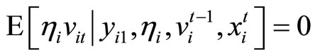 , (2.2.4)
where (2.2.4) is displayed for convenience, playing no role in constructing the valid moment conditions.
By replacing the unobservable variable  by the observable variable
  (which is written by using the dependent variables and the parameter of interest) in (2.2.1) - (2.2.3), the following Equations are obtained:
 , (2.2.5)
 (2.2.6)
 (2.2.7)
Utilizing the relationships holding among (2.2.5) - (2.2.7), the following ,
,  , and
, and  moment conditions are obtained:
 (2.2.8)
 (2.2.9)
 (2.2.10)
The moment conditions (2.2.8) are based on the relationships holding between  and
and  and holding between
  and
and  for
for , while the moment conditions (2.2.9) are based on the relationships holding between
  and
and . The moment conditions (2.2.10) are based on the relationships between
  and
and  for
for . The derivation of the moment conditions (2.2.8) - (2.2.10) is described in Appendix A.
The moment conditions (2.2.8) and (2.2.10) are the conventional moment conditions, which are linear with respect to  and based on the quasi-differencing transformation proposed by [2,3], while the moment conditions (2.2.9) are the additional moment conditions nonlinear with respect to
  on the basis of the covariance restrictions on the disturbances7.
In this paper, the moment conditions (2.2.8) and (2.2.10) are referred to as the quasi-differenced moment conditions by convention, while the moment conditions (2.2.9) are referred to as the additional nonlinear moment conditions.
It can be said that the quasi-differenced moment conditions and the additional nonlinear moment conditions correspond to the first-differenced moment conditions (otherwise known as the standard moment conditions) proposed by [25,26] and the additional nonlinear moment conditions proposed by [23,24] in the framework of the ordinary dynamic panel data model, respectively.
The moment conditions (2.2.8) and (2.2.9) are the condensed full set of the relationships holding among (2.2.5) and (2.2.6) in the sense that the other relationships are indirectly traced based on these relationships, while the moment conditions (2.2.10) are the condensed full set of the relationships found among (2.2.7).
2.3. Equidispersion and Moment Conditions
If the assumptions of the equidispersion are imposed on the LFM, the variance-covariance restrictions are produced by the addition of the following restrictions to the covariance restrictions (2.2.1) - (2.2.4):
 . (2.3.1)
By replacing the unobservable variable  by the observable variable
  in (2.3.1), the following Equations are obtained:
 . (2.3.2)
Utilizing the relationships holding among (2.2.6) and (2.3.2), the following two sets of  moment conditions are obtained:
 (2.3.3)
 (2.3.4)
The moment conditions (2.3.3) are based on the relationships holding between  and
and , while the moment conditions (2.3.4) are based on the relationships holding between
  and
and .
.
The moment conditions (2.3.3) are the additional moment conditions linear with respect to  for the case of the equidispersion, while the moment conditions (2.3.4) are the additional moment conditions nonlinear with respect to
 .
.
In this paper, the moment conditions (2.3.3) and (2.3.4) are referred to as the additional linear equidispersion moment conditions and the additional nonlinear equidispersion moment conditions, respectively.
The moment conditions (2.2.8), (2.3.3) and (2.3.4) are the condensed full set of the relationships holding among (2.2.5), (2.2.6) and (2.3.2) (i.e. the condensed full set when the equidispersion is assumed). The derivation of the moment conditions (2.3.3) and (2.3.4) is described in Appendix B.
2.4. Negbin I-Type Model and Moment Conditions
If the assumptions of the Negbin I-type model are imposed on the LFM, the variance-covariance restrictions are produced by the addition of the following restrictions to the covariance restrictions (2.2.1) - (2.2.4):
 . (2.4.1)
By replacing the unobservable variable  by the observable variable
  and the unobservable variable
 by the observable variable
 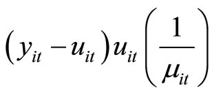 in
in
(2.4.1), the following Equations are obtained:
 8(2.4.2)
Utilizing the relationships holding among (2.2.6) and (2.4.2), the following two sets of  moment conditions are obtained:
 (2.4.3)
 (2.4.4)
The moment conditions (2.4.3) are based on the relationships holding between  and
and , while the moment conditions (2.4.4) are based on the relationships holding between
  and
and .
.
The moment conditions (2.4.3) are the additional moment conditions linear with respect to  for the case of the Negbin I-type model, while the moment conditions (2.4.4) are the additional moment conditions nonlinear with respect to
 .
.
In this paper, the moment conditions (2.4.3) and (2.4.4) are referred to as the additional linear Negbin I-type moment conditions and the additional nonlinear Negbin Itype moment conditions, respectively.
The moment conditions (2.2.8), (2.4.3) and (2.4.4) are the condensed full set of the relationships holding among (2.2.5), (2.2.6) and (2.4.2) (i.e. the condensed full set when the Negbin I-type model is assumed). The derivation of the moment conditions (2.4.3) and (2.4.4) is described in Appendix C.
2.5. Stationarity and Moment Conditions
The moment conditions concerning the stationarity are proposed and discussed in the ordinary dynamic panel data model (e.g. [24,28,29,31]). Likewise, they can be proposed in the LFM for count panel data.
If the explanatory variables  are stationary in terms of the moment generating functions as follows:
 (2.5.1)
(with  being any real number) and the initial condition of the count dependent variable is written as follows:
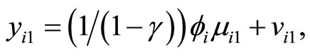 (2.5.2)
with
 (2.5.3)
the following  and
and  moment conditions are obtained by utilizing the relationships holding among (2.2.5) - (2.2.7):
 , (2.5.4)
 (2.5.5)
The moment conditions (2.5.4) are based on the relationships holding between  and
and  and holding between
  and
and , while the moment conditions (2.5.5) are based on the relationships holding between
  and
and  9. The moment conditions (2.5.4) for
  are the replacement of the moment conditions (2.2.9).
If the assumptions of the equidispersion are imposed in addition to those concerning the stationarity, the following  moment conditions are obtained by utilizing the relationships holding among (2.2.5), (2.2.6), and (2.3.2):
 (2.5.6)
Similarly, if the assumptions of the Negbin I-type model are imposed in addition to those concerning the stationarity, the following  moment conditions are obtained by utilizing the relationships holding among (2.2.5), (2.2.6), and (2.4.2):
 (2.5.7)
The moment conditions (2.5.6) and (2.5.7) for  are the replacement of the moment conditions (2.3.4) and (2.4.4), respectively.
The moment conditions (2.5.4) and (2.5.5) are the moment conditions concerning the stationarity on the basis of the covariance restrictions among the disturbances and between the regressors and the disturbances, respectively, while the moment conditions (2.5.6) and (2.5.7) are the moment conditions concerning the stationarity for the cases of the equidispersion and the Negbin I-type model, respectively. These moment conditions are linear with respect to .
.
In this paper, the moment conditions (2.5.4) and (2.5.5) are referred to as the stationarity moment conditions, while the moment conditions (2.5.6) and (2.5.7) are referred to as the stationarity & equidispersion moment conditions and the stationarity & Negbin I-type moment conditions, respectively.
It can be said that the stationarity moment conditions correspond to the stationarity moment conditions proposed by [28] and discussed by [24,29] in the framework of the ordinary dynamic panel data model.
When the stationarity is assumed, the moment conditions (2.2.8) and (2.5.4) are the condensed full set of the relationships holding among (2.2.5) and (2.2.6), while the moment conditions (2.2.10) and (2.5.5) are the condensed full set of the relationships holding among (2.2.7). The moment conditions (2.2.8), (2.3.3) and (2.5.6) are the condensed full set of the relationships holding among (2.2.5), (2.2.6) and (2.3.2) when the stationarity is assumed (i.e. the condensed full set when the stationarity and the equidispersion are assumed), while the moment conditions (2.2.8), (2.4.3) and (2.5.7) are the condensed full set of the relationships holding among (2.2.5), (2.2.6) and (2.4.2) when the stationarity is assumed (i.e. the condensed full set when the stationarity and the Negbin Itype model are assumed). The derivation of the moment conditions (2.5.4) - (2.5.7) is described in Appendix D.
2.6. GMM Estimator
Any set of the moment conditions for the LFM can be collectively written in the following  vector form:
 , (2.6.1)
where  is number of the moment conditions,
  ,
,  (which is the function of
 ) is composed of the observable variables and
  for the individual
 .
.
Using the following empirical counterpart for (2.6.1):
 , (2.6.2)
the GMM estimator  is constructed by minimizing the following criterion function with respect to
 :
:
 , (2.6.3)
where the  optimal weighting matrix is given as follows by using an initial consistent estimator of
  (i.e.
(i.e. ):
):
 . (2.6.4)
The efficient asymptotic variance for  is estimated by using
 , (2.6.5)
where . The GMM estimations for the LFM are explained in detail in [33,34].
Some GMM estimators are constructed for the LFM. The GMM estimators are classified into the three types.
First, the GMM estimators using the moment conditions linear with respect to  (without taking account of the stationarity) are presented: the GMM(QD) estimator using only the quasi-differenced moment conditions (i.e. (2.2.8) and (2.2.10)), the GMM(QDP) estimator using the quasi-differenced moment conditions and the additional linear equidispersion moment conditions (i.e. (2.3.3)), and the GMM(QDN) estimator using the quasi-differenced moment conditions and the additional linear Negbin Itype moment conditions (i.e. (2.4.3)).
Second, the GMM estimators using the condensed full sets of the moment conditions under the provided assumptions (without taking account of the stationarity) are presented: the GMM(PR) estimator using the quasi-differenced moment conditions and the additional nonlinear moment conditions (i.e. (2.2.9)), the GMM(PRP) estimator using the quasi-differenced moment conditions, the additional linear equidispersion moment conditions and the additional nonlinear equidispersion moment conditions (i.e. (2.3.4)), and the GMM(PRN) estimator using the quasi-differenced moment conditions and the additional linear Negbin I-type moment conditions and the additional nonlinear Negbin I-type moment conditions (i.e. (2.4.4)).
Third, the GMM estimators incorporating the moment conditions concering the stationarity are presented: the GMM(SA) estimator using the quasi-differenced moment conditions and the stationarity moment conditions (i.e. (2.5.4) and (2.5.5)), the GMM(SAP) estimator using the quasi-differenced moment conditions, the additional linear equidispersion moment conditions, the stationarity & equidispersion moment conditions (i.e. (2.5.6)) and the stationarity moment conditions with respect to  (i.e. (2.5.5)), and the GMM(SAN) estimator using the quasidifferenced moment conditions and the additional linear Negbin I-type moment conditions and the stationarity & Negbin I-type moment conditions (i.e. (2.5.7)) and the stationarity moment conditions with respect to
 .
.
It should be noted that there can be a case where a manipulation is needed, when using the additional nonlinear moment conditions, the additional nonlinear equidispersion moment conditions, the additional nonlinear Negbin I-type moment conditions, the stationarity moment conditions, the stationarity & equidispersion moment conditions, and the stationarity & Negbin I-type moment conditions for the GMM estimations. If all values in  are positive (which are commonplace in the empirical analysis), the GMM estimates of
  using these moment conditions seem to be in danger of going to infinity (see [3]). In this case,
  needs to be transformed in deviation from an appropriate value
 , in order that
  contains both positive and negative values evenly. The selection of
  by [30] is the overall mean of
  (i.e.
(i.e. 
 ). The GMM estimators subject to this transformation are the GMM(PR), GMM(PRP), GMM(PRN), GMM(SA), GMM(SAP), and GMM(SAN) estimators.
3. Monte Carlo
In this section, some small sample performances of the GMM estimators exhibited in previous section are investigated with Monte Carlo experiments. The experiments are implemented using the econometric software TSP version 4.5 (see [35]).
3.1. Data Generating Process
Two types of Data Generating Process (DGP) are configured: in one type, the dependent variables are generated from the Poisson distribution, while in another type, they are generated from the negative binomial distribution with the functional form being of the Negbin I-type.
The Poisson-type DGP is as follows:
 , (3.1.1)
 , (3.1.2)
 , (3.1.3)
 , (3.1.4)
 ;
; where
where  with
with  being the number of pre-sample periods to be generated. In the DGP, values are set to the parameters
 ,
,  ,
,  ,
,  ,
,  and
and . The experiments are carried out with
 , the cross-sectional sizes
 ,
,  and
and , the numbers of periods used for the estimations
 , and the number of replications
 . This DGP setting is the same as that of [1], except for the initial condition of
 . That is, the initial condition (3.1.2) denotes that the initial conditions of dependent variables are stationary and accordingly the dependent variables are in the stationary state if the absolute value of
  is less than one. The DGP is configured with the explanatory variables
  being strictly exogenous10.
In the Negbin I-type DGP, (3.1.1) and (3.1.2) are replaced by the following expressions respectively:
 , (3.1.5)
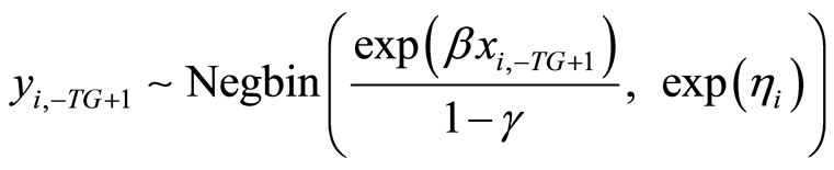 , (3.1.6)
where the denotation  implies that the count variable
  is distributed as the negative binomial distribution whose probability function is

with  being the gamma function and
  and
and  being the parameters with
  and
and  respectively.
3.2. Estimators for Comparison
The following three estimators are used for comparison: the Level estimator, the Within Group (WG) mean scaling estimator, and the PSM estimator. The Level and WG estimators are inconsistent in the DGP settings above. On the contrary, the PSM estimator is consistent if the long history is used in constructing the pre-sample means of the dependent variables. The details on these estimators are described in [1,10].
3.3. Results
For , Monte Carlo results for the Poisson-type DGP and the Negbin I-type DGP are shown in Table 1 and Table 2 respectively, while for
 , they are shown in Tables 3 and 4 respectively.


Table 1. Monte Carlo results for LFM, T = 4 (Poisson-type DGP).


Table 2. Monte Carlo results for LFM, T = 4 (Negbin I-type DGP).
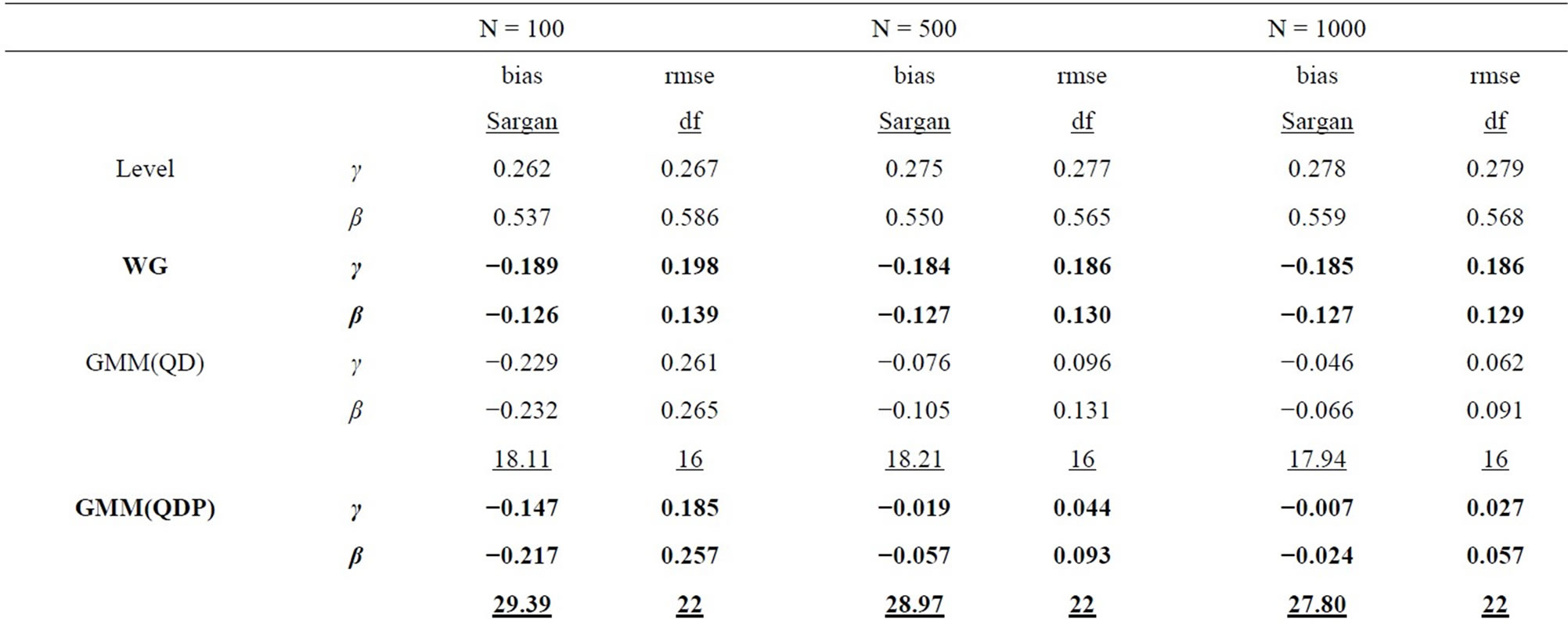


Table 3. Monte Carlo results for LFM, T = 8 (Poisson-type DGP).


Table 4. Monte Carlo results for LFM, T = 8 (Negbin I-type DGP).
In all tables, the endemic upward and downward biases are found for the Level and WG estimators respectively, while the PSM estimator behaves better as the longer pre-sample history is used. These results are almost the same as those obtained by [1].
It can be seen that the GMM estimators incorporating the additional moment conditions behave better than the GMM(QD) estimator using only the conventional moment conditions based on the quasi-differencing transformation, as long as the additional moment conditions are valid.
It is considered that the GMM(QD) estimator suffers from the weak instruments problem pointed out by [36,37], due to exclusively using the quasi-differenced moment conditions applying the lagged levels of dependent and explanatory variables (which are regarded as the weak instruments) to the quasi-differencing transformations (see, e.g., [1]). The weak instruments problem also occurs in the ordinary dynamic panel data model (see, e.g., [29]).
The small sample property of the distribution-free GMM estimator incorporating the additional nonlinear moment conditions (i.e. GMM(PR) estimator) is more preferable than that of the conventional GMM(QD) estimator. It can be said that the joint usage of the quasidifferenced moment conditions and the additional nonlinear moment conditions improves the small sample property of the GMM estimator, compared to the single usage of the quasi-differenced moment conditions. This result is similar to that for the ordinary dynamic panel data model (see, e.g., [38]).
For the Poisson-type DGP (see Table 1 and 3), the small sample properties of the GMM estimators incorporating the moment conditions associated with equidispersion (i.e. GMM(QDP), GMM(PRP), and GMM(SAP) estimators) improve as the cross-sectional size N increases from 100, 500 to 1000, while those of the GMM estimators incorporating the moment conditions associated with Negbin I-type model (i.e. GMM(QDN), GMM(PRN), and GMM(SAN) estimators) deteriorate, where the augmentations of the Monte Carlo means of Sargan test statistics (which are the reflection of the inconsistency) are recognizable for larger N. For the Negbin I-type DGP (see Tables 2 and 4), the countertrend is found. It is shown that each of both GMM estimators incorporating the moment conditions associated with equidispersion and incorporating those associated with the Negbin I-type model can discern each other’s underlying specification11.
The performances of the GMM estimators incorporateing the moment conditions concerning the stationarity (i.e. GMM(SA), GMM(SAP), GMM(SAN) estimators) are fairly favorable (especially in terms of bias), compared to that of the conventional GMM(QD) estimator, as long as the moment conditions used are valid. These results are similar to that for the ordinary dynamic panel data model, in which the additional usage of the sationarity moment conditions improves the small sample performance of the GMM estimator (see [29], etc.).
4. Conclusion
In this paper, some additional moment conditions other than the conventional quasi-differenced moment conditions were newly proposed for the LFM with explanatory variables being predetermined: the additional nonlinear moment conditions, the additional linear equidispersion moment conditions, the additional nonlinear equidispersion moment conditions, the additional linear Negbin Itype moment conditions, the additional nonlinear Negbin I-type moment conditions, the stationarity moment conditions, the stationarity & equidispersion moment conditions, and the stationarity & Negbin I-type moment conditions. In the limited Monte Carlo experiments, it was shown that the GMM estimators perform better when incorporating the additional moment conditions than when using the conventional moment conditions only, as long as the additional moment conditions are valid.
5. Acknowledgements
This paper is a collection of the oral presentations conducted in the 2008 International Symposium on Econometric Theory and Applications, Seoul National University (May 2008), the 2011 Asian Meeting of The Econometric Society, Korea University (August 2011), and the 18th International Panel Data Conference, Banque de France (July 2012). The presentations were also conducted in the domestic conferences in Japan: the meetings of The Japanese Economic Association (Kinki University, September 2008; Kwansai Gakuin University, September 2010), the meeting of The Japan Association for Applied Economics (Kobe University, November 2009), and the meeting of Kansai Keiryo Keizaigaku Kenkyukai (Kyoto University, January 2010) and in the seminars in Korea and Japan: Korea University (March 2008) and Kyushu University (June 2009). Author expresses the gratitude to the participants and the commentators: Kosuke Oya, Atsushi Fujii, and Atsushi Yoshida.
Appendix A
First, Equations (2.2.5) dated  and
and  give the following relationships:
 , (A.1)
 , (A.2)
while Equations (2.2.6) dated  and
and  for
for  give the following relationships:
 , (A.3)
 . (A.4)
Accordingly, subtracting (A.1) from (A.2), subtracting (A.3) from (A.4), and then taking notice of (2.1.1), the moment conditions (2.2.8) are obtained.
Second, Equations (2.2.6) dated  for
for  and
and  give the following relationships:
 , (A.5)
 . (A.6)
Accordingly, subtracting (A.6) from (A.5), the moment conditions (2.2.9) are obtained.
Third, Equations (2.2.7) dated  and
and  for
for  give the following relationships:
 (A.7)
(A.7)
 . (A.8)
Accordingly, subtracting (A.7) from (A.8), the moment conditions (2.2.10) are obtained.
Appendix B
First, Equation (2.3.2) dated  and Equation (2.2.6) dated
  for
for  give the following relationships:
 , (B.1)
 . (B.2)
Accordingly, subtracting (B.1) from (B.2) and then taking notice of (2.1.1) and (2.2.8), the moment conditions (2.3.3) are obtained.
Next, Equation (2.3.2) dated  and Equation (2.2.6) dated
  for
for  give the following relationships:
 , (B.3)
 . (B.4)
Accordingly, subtracting (B.4) from (B.3), the moment conditions (2.3.4) are obtained.
Appendix C
First, Equation (2.4.2) dated  and Equation (2.2.6) dated
  for
for  give the following relationships:
 (C.1)
(C.1)
 (C.2)
(C.2)
Accordingly, subtracting (C.1) from (C.2) and then taking notice of (2.1.1), (2.2.8) and the following moment conditions based on the transformation proposed by [3]:
 for
for  which are also valid for the LFM with explanatory variables being predetermined (i.e. (2.1.1) and (2.1.2) with (2.1.3)), the moment conditions (2.4.3) are obtained.
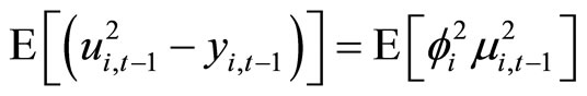
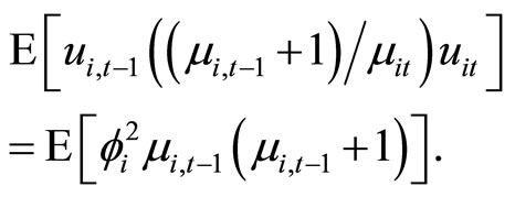
Next, equation (2.4.2) dated t and equation (2.2.6) dated t for  give the following relationships:
 (C.3)
(C.3)
 . (C.4)
Accordingly, subtracting (C.4) from (C.3), the moment conditions (2.4.4) are obtained.
Appendix D
First, allowing for the assumptions on the stationarity (i.e. (2.5.1) and (2.5.2) with (2.5.3)), Equation (2.2.5) dated  and Equations (2.2.6) dated
  for
for  and
and  give the following relationships:
 , (D.1)
 , (D.2)
 . (D.3)
Accordingly, using (D.1) - (D.3) and (2.1.1), the moment conditions (2.5.4) are obtained.
Second, allowing for the assumptions on the stationarity and utilizing the property of the moment generating function, Equations (2.2.7) dated  for
for  and
and  give the following relationships:
 , (D.4)
 , (D.5)
where . Accordingly, subtracting (D.4) from (D.5), the moment conditions (2.5.5) are obtained.
Third, allowing for the assumptions on the stationarity, Equation (2.3.2) dated  gives the following relationship:
 . (D.6)
Accordingly, using (D.1), (D.3), (D.6), (2.1.1) and (2.5.4), the moment conditions (2.5.6) are obtained.
Fourth, allowing for the assumptions on the stationarity, Equation (2.4.2) dated  gives the following relationship:
 (D.7)
(D.7)
Accordingly, using (D.1), (D.3), (D.7), (2.1.1) and (2.5.4), the moment conditions (2.5.7) are obtained.
Notes of Tables
NOTES
1Some trailblazing estimations of the knowledge production function using the quasi-differencing transformation are conducted by [7-9], etc.
2The origin of the PSM estimator can be traced to [11].
3The alternative models incorporating dynamics are proposed by [7,10].
4Some empirical works with respect to the knowledge production function applying these estimators to the LFM are conducted by [16-22], etc.
5Even if the long pre-sample histories of the dependent variables are available, the PSM estimator is not consistent unless the fixed effects composing the explanatory variables are proportional to the fixed effects in the regression and the (finite) moment generating functions of the disturbance terms composing the explanatory variables are equal over time and for all individuals.
6The terminology “Negbin I-type model” is used in [27].
7For the model without dynamics, variants of the moment conditions analogous to (2.2.9) are proposed by [30] for the case of endogenous regressors and by [7] for the case of strictly exogenous regressors, respectively. The former is valid for the case of predetermined regressors, while the latter is not.
8Note that
 taking notice of (2.1.1) and (2.1.2) with (2.1.3).
9Although author proposes the moment conditions (2.5.4) and (2.5.5) in the discussion paper of Kyushu Sangyo University in December, 2007, [32] also proposes the same moment conditions in the framework of a specification of the LFM slightly different from that in this paper. It can be said that [32] also makes some other contribution to the estimation of the LFM.
10[32] also conducts some Monte Carlo experiments in the similar setting.
11Although [39] proposes the moment condition based on the variancecovariance restrictions under the assumption with the explanatory variables being strictly exogenous and dynamics being excluded, it cannot distinguish between the equidispersion and the Negbin I-type model. However, it is shown that the moment conditions based on the variance-covariance restrictions proposed in this paper can distinguish between them, under the assumption weaker than [39].