1. Introduction
The derivation of Runge-Kutta schemes involving higher derivatives is now on the increase. Traditionally, given an initial value problem (IVP), classical explicit RungeKutta methods are derived with the intention of performing multiple evaluations of  in each internal stage for a given accuracy. Recently, Akanbi [1,2] derived multi-derivative explicit Runge-Kutta method involving up to second derivative. Goeken and Johnson [3] also derived explicit Runge-Kutta schemes of stages up to four with the first derivative of
 . However, the new scheme is derived with the notion of incorporating higher order derivatives of
  up to the second derivative. The cost of internal stage evaluations is reduced greatly and there is an appreciable improvement on the attainable order of accuracy of the method.
2. Derivation of the Proposed Scheme
The general form of a single step method for solving the Initial Value Problem (IVP)
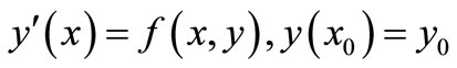 (1)
(1)
is defined as
 (2)
(2)
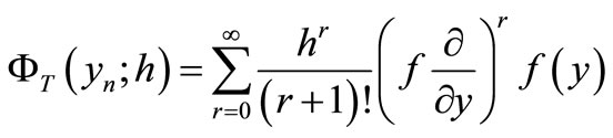
where  is obtained using the Taylor’s series expansion of an arbitrary function:
 (3)
(3)
and for the autonomous case of (1), in which ,
,  becomes
 (4)
(4)
The proposed scheme of this paper is of the form
 (5)
(5)
where
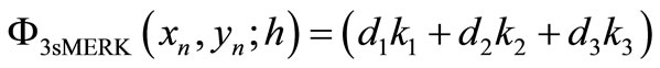 (6)
(6)


Expanding  and
and  in Taylor’s series and substituting the result into (5), the coefficients of the powers of
  are then compared with that of (3) to obtain the following system of equations:
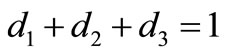


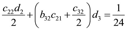


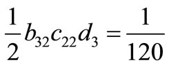


Solving the above system of equations, we have the set of solutions in Table 1.
The above solution set gives rise to a family of 3-stage multi-derivative explicit Runge-Kutta schemes. The proposed scheme denoted by 3sMERK above is thus given by


3. Convergence and Stability of the Method
3.1. Existence and Uniqueness of Solution
The properties of the incremental function  of the newly derived scheme are in general, very crucial to its stability and convergence characteristics [1,4-8].
Theorem 3.1.
Let , where
 , be defined and continuous for all
  in the region
  defined by
 , where a, b are finite, and let there exist a constant L such that
 (7)
(7)
holds every , then for any
 , there exist a unique solution
  of the problem (1), where
  is continuous and differentiable for all
 .
.
The requirement (7) is known as the Lipschitz’s condition, and the constant  is a Lipschitz’s constants [6, 7,9-11]. We shall assume that the hypothesis of this theorem is satisfied by the IVP (1). The following lemma will be useful for establishing the aforementioned characteristics.
Lemma 3.2.
Let  be a set of real numbers. If there exist finite constants
  and
and  such that
 (8)
(8)
then
 (9)
(9)
Proof. When , (9) is satisfied identically as
 .
.
Suppose (9) holds whenever  so that
 (10)
(10)
Then, from (8)  implies that
 (11)
(11)
On substituting (10) into (11), we have
 (12)
(12)
Hence, (9) holds for all .
. 
3.2. Accuracy and Stability
Usually, during the implementation of a computational scheme, errors are generated. The magnitude of the error determines how accurate and stable a scheme is. For instance, if the magnitude of the error is sufficiently small, the computational results would be accurate. However, if the magnitude of the error becomes so large, it can make the method unstable. The sources of error for these schemes and their principal error functions are discussed in Butcher [5,6], Fatunla [7] and Lambert [9, 10]. The following theorem guarantees the stability of the 3sMERK methods.
Theorem 3.3.
Suppose the IVP (1) satisfies the hypotheses of Theorem 3.1, then the new 3sMERK algorithm is stable.

Table 1. Examples of three-stage MERK methods.
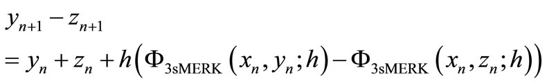
Proof. Let  and
and  be two sets of solutions generated recursively by the 3sMERK method with the initial condition
 , and
, and
 (13)
(13)
 (14)
(14)
 (15)
(15)
It implies that
Applying triangle inequality and (13), we have
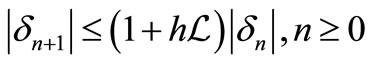
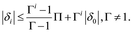
If we assume , and
, and , then Lemma 3.2 implies that
 , where
 . This implies the stability of the 3sMERK scheme.
4. Numerical Experiments
The proposed 3sMERK scheme (6) is applied to the two IVPs below and the results obtained are compared with the standard 3-stage methods of Runge-Kutta (Heun’s) [7,9,10] and that of Goeken and Johnson [3] stated in (16) and (17) respectively.
4.1. Heun’s Scheme
 (16)
(16)
4.2. Goeken’s Scheme
 (17)
(17)


Table 2. The absolute values of error of y(x) in Problem 1 using the proposed scheme and other methods, h = 0.001; 0.005; 0.025; 0.125.


Table 3. The absolute values of error of y(x) in Problem 2 using the proposed scheme and other methods, h = 0.001; 0.005; 0.025; 0.125.
4.3. Problem 1
Consider the IVP
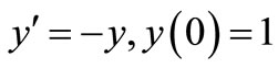 (18)
(18)
with the theoretical solution .
.
4.4. Problem 2
Consider the IVP
 (19)
(19)
with the theoretical solution
 .
.
5. Conclusions
The results generated by the proposed scheme in this paper when applied to the problems above, evidently proved the extent of accuracy of the scheme. Tables 2 and 3 above show the absolute error associated with the schemes for the test problems with the variation of the step length. The computations above clearly show the accuracy of the method. The standard Heun’s (third order) method grows faster in error than the method of Goeken and the newly derived scheme. However, 3sMERK performed best among the three methods.
Based on the two problems solved above, it follows that the scheme is quite efficient. We therefore conclude that the 3sMERK method proposed is reliable, stable and with high accuracy.
NOTES