Portfolio Size in Stochastic Portfolio Networks Using Digital Portfolio Theory ()
1. Introduction
The choice of financial risk measures is very important in the assessment of the riskiness of financial positions. For this reason, several classes of financial risk measures have been proposed in the literature. Among these are coherent and convex risk measures, Choquet expectations and Peng’s g-expectations. Coherent risk measures were first introduced by Artzner, Delbaen, Eber and Heath [1] and Delbaen [2]. As an extension of coherent risk measures, convex risk measures in general probability spaces were introduced by Föllmer & Schied [3] and Frittelli & Rosazza Gianin [4]. g-expectations were introduced by Peng [5] via a class of nonlinear backward stochastic differential equations (BSDEs), this class of nonlinear BSDEs being introduced earlier by Pardoux and Peng [6]. Choquet [7] extended probability measures to nonadditive probability measures (capacity), and introduced the so called Choquet expectation.
Our interest in this paper is to explore the relations among risk measures and expectations. To do so, we restrict our attention of coherent and convex risk measures and Choquet expectations to the domain of g-expectations. The distinctions between coherent risk measure and convex risk measure are accounted for intuitively in the framework of g-expectations. We show that 1) in the family of convex risk measures, only coherent risk measures satisfy Jensen’s inequality; 2) coherent risk measures are always bounded by the corresponding Choquet expectation, but such an inequality in general fails for convex risk measures. In finance, coherent and convex risk measures and Choquet expectations are often used in the pricing of a contingent claim. Result 2) implies coherent pricing is always less than Choquet pricing, but the pricing by a convex risk measure no longer has this property. We also study the relation between static and dynamic risk measures. We establish that if g-expectations are coherent (convex) risk measures, then the same is true for the corresponding conditional g-expectations or dynamic risk. In order to prove these results, we establish in Section 3, Theorem 1, a new converse comparison theorem of g-expectations. Jiang [8] studies gexpectation and shows that some cases give rise to risk measures. Here we are able to show, in the case of gexpectations, that coherent risk measures are bounded by Choquet expectation but this relation fails for convex risk measures; see Theorem 4. Also we show that convex risk measures obey Jensen’s inequality; see Theorem 3.
The paper is organized as follows. Section 2 reviews and gives the various definitions needed here. Section 3 gives the main results and proofs. Section 4 gives a summary of the results, putting them into a Table form for convenience of the various relations.
2. Expectations and Risk Measures
In this section, we briefly recall the definitions of g-expectation, Choquet expectation, coherent and convex risk measures.
2.1. g-Expectation
Peng [5] introduced g-expectation via a class of backward stochastic differential equations (BSDE). Some of the relevant definition and notation are given here.
Fix  and let
  be a
be a  -dimensional standard Brownian motion defined on a completed probability space
 . Suppose
  is the natural filtration generated by
 , that is
  We also assume
 . Denote


Let 
 satisfy
(H1) For any  is a continuous progressively measurable process with
 .
.
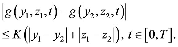
(H2) There exists a constant  such that for any

(H3) 
In Section 3, Corollary 3 we will consider a special case of  with
with .
.
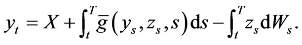
Under the assumptions of (H1) and (H2), Pardoux and Peng [6] showed that for any , the BSDE
 (1)
(1)
has a unique pair solution
 .
.
Using the solution  of BSDE (1), which depends on
 , Peng [5] introduced the notion of g-expectations.
Definition 1 Assume that (H1), (H2) and (H3) hold on g and . Let
. Let  be the solution of BSDE (1).
 defined by
  is called the g-expectation of the random variable
 .
.
 defined by
  is called the conditional g-expectation of the random variable
 .
.
Peng [5] also showed that g-expectation  and conditional
  -expectation
  preserve most of basic properties of mathematical expectation, except for linearity. The basic properties are summarized in the next Lemma.
Lemma 1 (Peng) Suppose that
 .
.
1) Preservation of constants: For any constant 
 .
.
2) Monotonicity: If , then
 .
.
3) Strict monotonicity: If , and
, and , then
 .
.
4) Consistency: For any ,
,
 .
.
5) If  does not depend on
 , and
, and  is
is  - measurable, then

In particular, .
.
6) Continuity: If  as
as  in
in , then
 .
.
The following lemma is from Briand et al. [9, Theorem 2.1]. We can rewrite it as follows.
Lemma 2 (Briand et al. ) Suppose that  is of the form
 where
where  is a continuous bounded process. Then

where the limit is in the sense of .
.
2.2. Choquet Expectation
Choquet [7] extended the notion of a probability measure to nonadditive probability (called capacity) and defined a kind of nonlinear expectation, which is now called Choquet expectation.
Definition 2
1) A real valued set function  is called a capacity if a)
b) , whenever
  and
and .
.
2) Let  be a capacity. For any
 , the Choquet expectation
  is defined by

Remark 1 A property of Choquet expectation is positive homogeneity, i.e. for any constant 

2.3. Risk Measures
A risk measure is a map  where
where  is interpreted as the “habitat” of the financial positions whose riskiness has to be quantified. In this paper, we shall consider
 .
.
The following modifications of coherent risk measures (Artzner et al.[1]) is from Roorda et. al. [10].
Definition 3 A risk measure  is said to be coherent if it satisfies 1) Subadditivity:
 ,
, ;
;
2) Positive homogeneity:  for all real number
3) Monotonicity:  whenever
4) Translation invariance:  for all real number
 .
.
As an extension of coherent risk measures, Föllmer and Schied [3] introduced the axiomatic setting for convex risk measures. The following modifications of convex risk measures of Föllmer and Schied [3] is from Frittelli and Rosazza Gianin [4].
Definition 4 A risk measure is said to be convex if it satisfies 1) Convexity:
 ,
,

 ;
;
2) Normality: ;
;
3) Properties (3) and (4) in Definition 3.
A functional  in Definitions 3 and 4 is usually called a static risk measure. Obviously, a coherent risk measure is a convex risk measure.
As an extension of such a functional  Artzner et al. [11,12], Frittelli and Rosazza Gianin [13] introduced the notion of dynamic risk measure
  which is random and depends on a time parameter
 .
.
Definition 5 A dynamic risk measure

is a random functional which depends on , such that for each
  it is a risk measure. If
  satisfies for each
  the conditions in Definition 3, we say
  is a dynamic coherent risk measure. Similarly if
  satisfies for each
  the conditions in Definition 4, we say
  is a dynamic convex risk measure.
3. Main Results
In order to prove our main results, we establish a general converse comparison theorem of g-expectation. This theorem plays an important role in this paper.
Theorem 1 Suppose that  and
and  satisfy (H1), (H2) and (H3). Then the following conclusions are equivalent.
1) For any 

2) For any 
 (2)
(2)
Proof: We first show that inequality (2) implies inequality 3).
Let 
 and
and  be the solutions of the following BSDE corresponding to the terminal value
  and
and  and the generator
  and
and , respectively
 (3)
(3)
Then 


For fixed , consider the BSDE
 (4)
(4)
It is easy to check that  is the solution of the BSDE (4).
Comparing BSDEs (4) and (3) with  and
and , assumption (2), (2) then yields

Applying the comparison theorem of BSDE in Peng [5], we have  Taking
 , thus by the definition of
  -expectation, the proof of this part is complete.
We now prove that inequality (1) implies (2). We distinguish two cases: the former where  does not depend on
 , the latter where
  may depend on
 .
.
Case 1,  does not depend on
 . The proof of this case 1 is done in two steps.
Case 1, Step 1: We now show that for any , we have

Indeed, for , set
, set

If for all , we have
  then we obtain our result.
If not, then there exists  such that
 . We will now obtain a contradiction.
For this ,
,

That is

Taking g-expectation on both sides of the above inequality, and apply the strict monotonicity of  -expectation in Lemma 1 (3), it follows

But by Lemma 1 (4) and (5),

Note that by Lemma 1(v)

Thus

This induces a contradiction, thus concluding the proof of this Step 1.
Case 1, Step 2: For any  with
with  and
and , let us choose
 . Obviously,
By Step 1,

Thus

Let  applying Lemma 2, since g does not depend on
  we rewrite
  simply as
  thus
thus  The proof of Case 1 is complete.
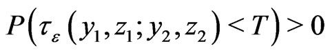
Case 2, g depends on y. The proof is similar to the proof of Theorem 2.1 in Coquet et al. [14]. For each  and
and  define the stopping time

Obviously, if for each 
 , for all
  then the proof is done. If it is not the case, then there exist
  and
and

such that
 .
.
Fix  and consider the following (forward) SDEs defined on the interval
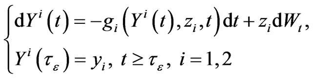
and

Obviously, the above equations admit a unique solution  which is progressively measurable with

Define the following stopping time

It is clear that  and note that
  whenever
  thus,
thus, 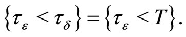 Hence
Hence .
.
Moreover, we can prove

In fact, setting
 then
then

Thus 
It follows that on ,
,  This implies
 (5)
(5)
By the definition of  and
and , the pair processes
  and
and  are the solutions of the following BSDEs with terminal values
 and
and ,
,

and

Hence,


and

Applying the strict comparison theorem of BSDE and inequality (5), by the assumptions of this Theorem, we have

This induces a contradiction. The proof is complete.
Lemma 3 Suppose that g satisfies (H1), (H2) and (H3). For any constant , let
, let
 .
.
Then for any ,
, 
Proof: Letting , then
  is the solution of BSDE

Since
 the above BSDE can be rewritten as
 (6)
(6)
Let , then
  satisfies
 (7)
(7)
Comparing with BSDE (6) and BSDE (7), by the uniqueness of the solution of BSDE, we have

Let  then
then . The conclusion of the Lemma now follows by the definition of g-expectation. This concludes the proof.
Applying Theorem 1 and Lemma 3, immediately, we obtain several relations between g-expectation  and
and . These are given in the following Corollaries.
Corollary 1 The g-expectation  is the classical mathematical expectation if and only if g does not depend on
  and is linear in
 .
.
Proof: Applying Theorem 1,  is linear if and only if
  is linear in
 . By assumption (H3), that is
  for all
 . Thus
  does not depend on
 . The proof is complete.
Corollary 2 The  -expectation
  is a convex risk measure if and only if
  does not depend on
  and is convex in
 .
.
Proof: Obviously,  -expectation
  is convex risk measure if and only if for any
 (8)
(8)
For a fixed , let
, let

Applying Lemma 3,

Inequality (8) becomes

Applying Theorem 1, for any


which then implies that g is convex. By the explanation of Remark for Lemma 4.5 in Briand et al. [9], the convexity of  and the assumption (H3) imply that
  does not depend on
 . The proof is complete.
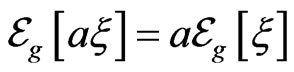
The function  is positively homogeneous in
  if for any
 ,
, .
.
Corollary 3 The  -expectation
  is a coherent risk measure if and only if
  does not depend on
  and it is convex and positively homogenous in
 . In particular, if
 ,
,  is of the form
 with
with .
.
Proof: By Corollary 2, the  -expectation
  is a convex risk measure if and only if
  does not depend on
  and is convex in
 . Applying Theorem 1 and Lemma 3 again, it is easy to check that
  -expectation
  is positively homogeneous if and only if
  is positively homogeneous (that is for all
  and
and 
 if and only if for any
 ,
, .
.
In particular, if , notice the fact that
  is convex and positively homogeneous on
 , and that
  does not depend on
 . We write it as
  then
then
 (9)
(9)
Note that ,
,  , but
, but

Thus from (9)

Defining
 ,
, .
.
Obviously  since the convexity of
  yields

The proof is complete.
Remark 2 Corollaries 2 and 3 give us an intuitive explanation for the distinction between coherent and convex risk measures. In the framework of g-expectations, convex risk measures are generated by convex functions, while coherent measures are generated only by convex and positively homogenous functions. In particular, if d = 1, it is generated only by the family  with
with . Thus the family of coherent risk measures is much smaller than the family of convex risk measures.
Jensen’s inequality for mathematical inequality is important in probability theory. Chen et al. [15] studied Jensen’s inequality for g-expectation.
We say that  -expectation satisfies Jensen’s inequality if for any convex function
  then
then
 (10)
(10)
Lemma 4 [Chen et al. [15] Theorem 3.1] Let  be a convex function and satisfy
 ,
,  and
and . Then 1) Jensen’s inequality (10) holds for
  -expectations if and only if
  does not depend on
  and is positively homogeneous in
 ;
;
2) If  the necessary and sufficient condition for Jensen’s inequality (10) to hold is that there exist two adapted processes
  and
and  such that
 .
.
Now we can easily obtain our main results. Theorem 2 below shows the relation between static risk measures and dynamic risk measures.
Theorem 2 If  -expectation
  is a static convex (coherent) risk measure, then the corresponding conditional g-expectation
  is dynamic convex (coherent) risk measure for each
Proof: This follows directly direct from Theorem 1.
Theorem 3 below shows that in the family of convex risk measure, only coherent risk measure satisfies Jensen’s inequality.
Theorem 3 Suppose that  is a convex risk measure. Then
  is a coherent risk measure if and only if
  satisfies Jensen’s inequality.
Proof: If  is a convex risk measure, then by Corollary 2,
  is convex. Applying Lemma 4,
  satisfies Jensen’s inequality if and only if
  is positively homogenous. By Corollary 2, the corresponding
  is coherent risk measure. The proof is complete.
Theorem 4 and Counterexample 1 below give the relation between risk measures and Choquet expectation.
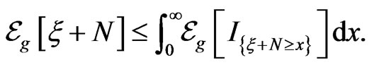
Theorem 4 If  is a coherent risk measure, then
  is bounded by the corresponding Choquet expectation, that is
  where
where . If
. If  is a convex risk measure then inequality above fails in general. By construction there exists a convex risk measure and random variables
  and
and  such that

The prove this theorem uses the following lemma.
Lemma 5 Suppose that  does not depend on
 . Suppose that the
  -expectation
  satisfies (1)
  (2) For any positive constant
 ,
,

Then for any  the
the  -expectation
  is bounded by the corresponding Choquet expectation, that is
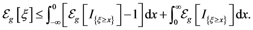 (11)
(11)
Proof: The proof is done in three steps.
Step 1. We show that if  is bounded by
 , then inequality (11) holds.
In fact, for the fixed , denote
  by
by

Then  in
in 
Moreover,  can be rewritten as

But by the assumptions (1) and (2) in this lemma, we have
 (12)
(12)
Note that

and 
Thus, taking limits on both sides of inequality (12), it follows that  The proof of Step 1 is complete.
Step 2. We show that if  is bounded by
 , that is
 , then inequality (11) holds.
Let  then
then  Applying Step 1,
 (13)
(13)
But by Lemma 1(v),  On the other hand,

Thus by (13)

Therefore

Step 3. For any  let
let  then
then . By Step 2,

Letting , it follows that

The proof is complete.
Proof of Theorem 4: If the  -expectation
  is a coherent risk measure, then it is easy to check that the
  -expectation
  satisfies the conditions of Lemma 5.
Let 
 . By Lemma 5 and the definition of Choquet expectation, we have
  The first part of this theorem is complete.
Counterexample 1 shows that this property of coherent risk measures fails in general for more general convex risk measures. This completes the proof of Theorem 4.
Counterexample 1 Suppose that  is 1-dimensional Brownian motion (i.e. d = 1). Let
 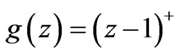 where
where . Then
  is a convex risk measure. Let
  and
and  Then
Then
 However
  Here the capacity
  in the Choquet expectation
  is given by
Proof of the Inequality in Counterexample 1: The convex function  satisfies (H1), (H2) and(H3). Thus, by Corollary 2,
  -expectation
  is a convex risk measure. This together with the property of Choquet expectation in Remark 1 implies

Moreover, since  by Corollary 3,
  is a convex risk measure rather than a coherent risk measure. We now prove that
  In fact, since

we only need to show

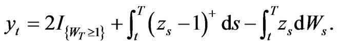
Let  be the solution of the BSDE
 (14)
(14)
First we prove that
 (15)
(15)
where  is Lebesgue measure on
If it is not true, then  a.e.
a.e.  and BSDE (14) becomes

Thus

By the Markov property,

Recall that  and
and  are independent and
 . Thus

where  is the density function of the normal distribution
 . Thus
  where
where  is the Malliavin derivative. Thus
  can be greater than 1 whenever
  is near 0 and
  is near 0. Thus (15) holds, which contradicts the assumption
  a.e.
a.e. .
.
Secondly we prove that

Let  be the solution of the BSDE
 (16)
(16)
Obviously,

which means  is the solution of BSDE

But  Thus by the uniqueness of the solution of BSDE,
  On the other hand, let
  be the solution of the BSDE
 (17)
(17)
Comparing BSDE(17) with BSDE (16), notice (15) and the fact
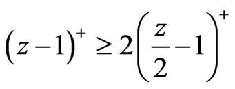 and
and 
whenever z >1. By the strict comparison theorem of BSDE, we have 
Setting , thus

The proof is complete.
Remark 3 In mathematical finance, coherent and convex risk measures and Choquet expectation are used in the pricing of contingent claim. Theorem 4 shows that coherent pricing is always less than Choquet pricing, while Counterexample 1 demonstrates that pricing by a convex risk measure no longer has this property. In fact the convex risk price may be greater than or less than the Choquet expectation.
4. Summary
Coherent risk measures are a generalization of mathematical expectations, while convex risk measures are a generalization of coherent risk measures. In the framework of  -expectation, the summary of our results is given in Table 1. In that Table, the Choquet expectation is
 .
.
Counterexample 1 shows that convex risk may be  or
or  Choquet expectation. Only in the case of coherent

Table 1. Relations among coherent and convex risk measures , choquet expectation and Jensen’s inequality.
risk there is an inequality relation with Choquet expectation.
NOTES
This work has been supported by grants from the Natural Sciences and Engineering Research Council (NSERC) of Canada.