Endogenous Stock Market Participation and Wealth Accumulation: A Life-Cycle Model Perspective

Dongxu Li, Steve Yang^*

School of Business, Stevens Institute of Technology, Hoboken, NJ, USA.

DOI: 10.4236/tel.[phone]                

Abstract

We propose a life-cycle model, where individuals facing uninsured labor income risks choose whether to participate in the stock market and make decisions on home ownership, in an environment with a social safety net and the retirement savings system. The model is motivated by the empirical finding that active stock market participation is associated with higher education and employment experience in the finance sector. The model exhibits a good fit on portfolio choice, home ownership, and consumption patterns in the cross-section and through the life cycle. The lack of stock market access, approximated by a fixed entry cost and variable costs, plays a crucial role in generating heterogeneous outcomes in agents’ wealth accumulation, increasing wealth inequality.

Keywords

Life-Cycle Model, Household Finance, Stock Market Participation, Financial Literacy

1. Introduction

The recent emergence of the online trading platform Robinhood and the GameStop stock price surge mania might mislead people into thinking that access to the equity market is ubiquitous. In fact, this is a relatively new phenomenon. It is well known in the finance and economics literature that only a small fraction of the population actively participated in the stock market outside of their retirement savings account. This phenomenon is puzzling since in the long run the stock returns are significantly higher than risk-free bonds—some scholars view the “participation puzzle” as the extensive margin version of the “equity premium puzzle”¹.

Motivated by the empirical evidence that heterogeneity in education and finance work experience creates diverging wealth growth paths, we build a life-cycle model where agents endogenously choose whether to participate in the stock market investment. We study this calibrated life-cycle model where we allow agents to be endowed with different levels of earning power and different costs of stock market access. We then examine the question of how stock market participation would influence agents’ wealth accumulation and understand how much of the observed wealth inequality can be attributed to the lack of equity market access, or the difficulty of acquiring such access.

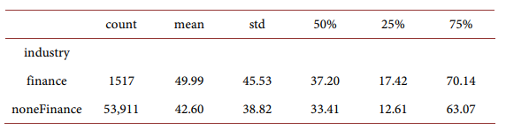
To give credence to our model assumptions, we first document and confirm, using the Panel Study of Income Dynamics (PSID) data, that stock market participation and stock investment level are associated with a higher level of education and employment experience in the finance sector. The former can be interpreted as having higher earning power, while the latter can be interpreted as having the basic knowledge of investment under uncertainty and understanding risk-return trade-offs in the equity market. According to the empirical analysis, having a college degree or above, on average, is associated with an 11% higher participation probability, a higher investment amount of 89k, and a higher total wealth of 49k than those who don’t have a college degree. A similar analysis also reveals that employment experience in the finance industry is associated with 7% higher participation probability, 32k higher investment amount, and 10k higher total wealth than those who do not have finance industry experience.

Motivated by the empirical evidence, we specify a model where agents, with a goal of maximizing the accumulated utility—the desired level of well-being, make consumption and savings decisions throughout each period in their life cycle. In this partial equilibrium model, agents make savings and consumption decisions under an uncertain economic environment and are subject to several uninsured risks such as unemployment and mortality. With our model setting, agents can save through the risk-free bond market. Agents may also choose to access the stock market for a higher but more volatile return. However, agents need to pay a fixed entry cost upfront and incur variable costs for participating in the stock market. Agents are ex-ante heterogeneous in their earning power and finance experience, and the finance experience is associated with lower stock market entry costs. A natural implication of the model is that stock market participation and the investment amount are higher in agents with higher earning power and are more financially literate. The model exhibits a good fit on key life-cycle moments observed in the PSID data such as the earnings profile, the hump-shaped consumption profile, stock investment amount, the total liquid wealth, home-ownership rates, etc.

The model is also rich in features. First of all, the agents participate in the labor market and face both aggregate and idiosyncratic risks which affect their income level and employment status. Second, in addition to non-durable goods consumption, the agents also derive utility from housing consumption through renting or home ownership. Home purchases require a down payment and taking out a mortgage, the interest portion of which is tax-deductible. Third, the agents are saving for retirement in a tax-advantaged account and can only withdraw from that account after retirement. Adding large and predictable expenditures into the life-cycle model affects the timing and amount of stock market investments. For instance, if a young agent were to save for a down payment for a home purchase, it would affect his/her willingness to take risks in the stock market. The safety net that the retirement savings account provides would also reduce the incentive for the agents to save in the form of liquid wealth investments.

Our paper makes three major contributions to the current literature. First, with a set of empirical analyses, we find that education, employment experience in the finance industry, retirement status, and home ownership are all positively predicting agents’ stock market participation, investment amount, and total wealth. Most importantly, on average, having a college degree is associated with an 11% increase in participation probability, while working in the finance industry increases an agent’s participation probability by 7%. Second, we build a feature-rich structural life-cycle model to investigate household financial decisions. Setting in a partial equilibrium, agents take aggregate asset returns and macroeconomic conditions as given and make consumption and investment decisions accordingly. When we calibrate the model parameters using otherwise standard procedures in macrofinance, our baseline model exhibits a good fit on several key empirical observations such as portfolio choice, home ownership, and consumption pattern in the cross-section and through the life-cycle. Finally, our simulation study finds that the lack of stock market access, approximated by participation costs, plays a key role in generating heterogeneous outcomes in agents’ wealth accumulation, increasing wealth inequality. This finding is supported by the following two counterfactual experiments. First, on average, a person with high earning power and regular access to the stock market accumulates, at age 50, $35.49K or 39.45% more wealth and becomes a home-owner 3 years sooner, relative to a person with the same earning power but high stock market participation cost. Second, on average, a person with low earning power would accumulate, at age 50, $23.44k or 135.23% more wealth, if they are given easier access to the equity market. The overall home-ownership rate would have been increased by 16% as well. These results indicate that participation cost plays a crucial role in agents’ wealth accumulation.

The life-cycle modeling approach has a long tradition in economics and can trace back its roots to Fisher’s finite horizon model Fisher (1930) . Compared with canonical models in macroeconomics featuring infinitely-lived agents, this class of models offers a more realistic way to study education, retirement, financial investment, and home ownership. One of the earlier works by Jagannathan et al. (1996) assesses the portfolio choice of the old versus the young and stresses the key role played by the labor income process. Cagetti (2003) provides a very comprehensive modeling of the income process and studies the importance of precautionary savings in a life-cycle model featuring heterogeneity in age and education. Arellano et al. (2017) focuses on the interaction between earning and consumption dynamics. Using the same life-cycle modeling setup, Huggett et al. (2011) investigate the relative importance of idiosyncratic shocks (luck) versus initial conditions in contributing to lifetime income and wealth inequality and provide evidence in favor of luck.

Our work is closely related to the following three papers: Gomes and Michaelides (2005) , Wong (2015) , and Vestman (2019) . Gomes and Michaelides (2005) study life-cycle asset allocation and successfully generate non-participation in a model by allowing for heterogeneity in risk aversion, without explicitly modeling major life-cycle events such as home ownership and individual retirement account. Vestman (2019) studies a life-cycle portfolio choice model with endogenous housing choice. The primary focus of that is to explain the higher stock market participation rates amongst homeowners. In his paper, agents have different preferences over risk aversion and elasticity of inter-temporal substitution (EIS). Agents with strong saving motives self-select to become homeowners and invest more in the equity market. In this paper, rather than assuming agents have heterogeneous preferences, we focus on the positive relationship between high earning power and easy access to the equity market. Another key difference lies in the different approaches to modeling home ownership. Vestman (2019) allows the agent to switch in and out of home ownership but keeps the level of home equity constant. In our model environment, we allow agents to “fire sale” their homes only in the event of financial distress. On the other hand, we allow agents to accumulate home equity over time and increase their total wealth through home ownership. The approach we follow in modeling housing is influenced by Wong (2015) , which develops a life-cycle model that allows agents to flexibly buy, sell, and refinance their homes, and use this model to study the heterogeneous consumption responses to monetary policy shocks amongst people at different points in their life-cycle. We extend the framework of Wong (2015) by considering stock market participation and retirement savings in agents’ life-cycle decisions.

The second string of related literature is the effect of financial literacy, home equity, and the relationship between labor market skill, financial literacy, and stock market participation cost. Zhu (2019) finds empirical results showing that the increase in net housing value will significantly increase the proportion of households participating in the stock market and the shareholding rate. Delavande et al. (2008) use a simple two-period model of consumer saving and portfolio allocation across safe bonds and risky stocks and show that individuals will optimally choose to invest in financial knowledge to gain access to higher-return assets. Using Dutch survey data, van Rooij et al. (2011) finds that financial literacy increases with people’s educational attainment, and those who lack financial literacy are much less likely to invest in stocks. Xie (2021) seeks to determine the correlations between financial literacy, family income, and fiscal prudence, and study the difference in financial behavior among young adults from privileged and common families. Bernheim and Garrett (2003) use survey data to show that education in financial literacy at the workplace increases investment in the stock market. One theoretical interpretation, as summarized by Hong et al. (2004) is that education reduces the fixed cost of participation. The more financially literate investors are, the better they understand the risk-reward trade-offs. They find it less costly in terms of time, attention, and resources when setting up accounts and executing trades. The presence of market frictions mostly in the form of fixed entry and/or transaction costs offers promising explanations for the limited stock market participation, Alan (2006) built a structural model to estimate a one-time entry cost of approximately 2 percent of annual permanent income. Recently, Athreya et al. (2015) explored in a Ben-Porath (1967) —style human capital investment model, the endogenous relationship between labor market skill and participation. They show that agents with high learning ability choose to invest in their financial literacy², and increased their stock market investment. We kept such endogenous mechanisms in mind but took the connection between skill and financial literacy as exogenously given and explored its implications.

A well-calibrated life-cycle model also serves as a good building block for the equilibrium asset pricing literature. In this literature, one way to generate high and volatile equity premiums with smooth macroeconomic fundamentals is to prevent some agents from investing in the stock market. For example, in Guvenen (2009) , agents are infinitely lived and some agents are exogenously excluded from the equity market, shifting the market risk to agents who participate. A potential shortcoming of this approach is that participation status is exogenous and predetermined. We think of our current life-cycle model as potentially a good candidate work-horse to place in the general equilibrium framework.

The rest of the paper is organized as follows: Section 2 presents data and empirical analysis. Section 3 introduces the life-cycle model. Section 4 discusses the calibration of the model and shows the model’s simulation experiments, implications, and variations. Section 5 concludes the paper and points to some future extensions.

2. Empirical Evidence

2.1. Determinants of Active Stock Market Participation

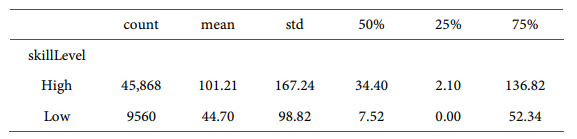
Our empirical analysis is based on the Panel Study of Income Dynamics (PSID) dataset³. We use around 60,000 data points from a repeated cross-section of U.S. families between 1999 and 2019. This is a survey-based dataset, where respondents are asked whether they have actively participated in the stock market and if so, how much is invested in the stock market. The respondents also answered questions regarding their income, liquid wealth, home equity, and total wealth. We converted all monetary amounts into the dollar value in 2005 (inflation adjustment)⁴. For regression analysis, we filter out extreme values in wealth and income. In addition, for each agent, we can also observe a set of demographic information, such as age, gender, employment status, education attainment, occupation, and industry they have worked in. In the entire sample, only 16% percent of the respondents invest actively in the stock market, which we define as a direct investment through a brokerage account, as opposed to passive and indirect investment through a retirement account or an asset management firm. The low level of participation is partly a result of the time period we have covered. In fact, the participation rate was 23% in 1999, 17% in 2009, and 11% in 2019, reflecting that there are secular trends in stock market participation (See Table 1).

We report participation rates by demographic groups. We do so by focusing on a family whose head of the household is between 20 and 80 years old and dividing them into three groups, i.e. Young (20 - 40), Mid-aged (41 - 60), and Old (61 and above). As shown in Figure 1(a), participation amongst the young is relatively low around 12%, increased to around 18% for mid-aged people, and closing in at around 25% for the elderly.

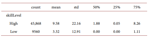
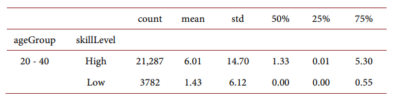
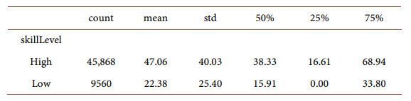
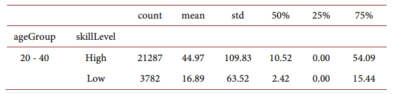
We report stock market participation by different levels of educational attainment in Figure 1(b) and note that amongst people without a college degree, participation is only 4% percent, while amongst people with a college degree participation percentage is around 11%. Stock market participation is highest amongst people with a post-graduate education, which is around 30%. For our regression analysis, we categorize households into “high-skill” households if the head of the household attained a postgraduate degree and “low-skill” households otherwise. Figure 2 shows that “high-skill” households’ labor income tends to outperform the “low-skill” households and accumulated much more wealth on average through their life cycle.

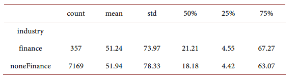
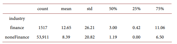
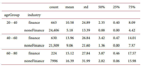
We investigate whether historical employment in the broadly defined finance industry is associated with a higher participation rate. As we can see in Figure 3(a), over 25 percent of workers with finance-related work experience participate in the stock market, which is higher than the workers without such experiences. If we take a closer look at the households who are financially literate (indicating easier access to the stock market), over 55% of them are “high-skill” households (as shown in Figure 3(b)). Intuitively, people with higher earning power are also more likely to be financially literate.

Table 1. Participation through time.

Figure 1. Age and education.

Figure 2. Wealth and income on education.

Figure 3. Finance related work experience.

We finally turn our attention to the participation ratio by employment status. We assign people in our sample to three possible employment statuses: employed, unemployed, and those who are not in the labor force. We observed that retired people have a larger chance of participating in the stock market, as over 25% of them do (see Figure 4). And house owners seem to be more active in stock investment. An additional set of summary statistics tables are reported in the appendix.

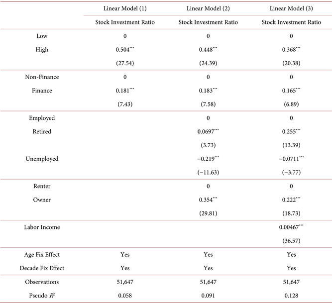
To get a holistic view of the determinants of stock market participation, we run a set of logistic regressions to simultaneously account for the role of education, employment status, and occupation in determining people’s participation decisions in the stock market. In these regressions, the dependent variable takes the binary value 1 or 0, indicating either participation or no participation in the stock market. The independent variables are categorical variables including the “skill level”, employment status, home status, and finance industry employment. Table 2 and Table 3 report the summary statistics for qualitative variables and quantitative variables used in these analyses, respectively.

For ease of interpretation, we report the average marginal effect of the variables and the coefficient estimates of the logistic regression in Table 4. In all three specifications presented here, we include educational attainment and the finance industry dummies as predictors and control for age and decade-related fixed effects. On average, having a college degree is associated with an 11% increase in participation probability, while working in the finance industry increases participation probability by 6.7%. Specifications (2) and (3) control for employment status and

Figure 4. Participation ratio in home ownership.

Table 2. Qualitative variables used in regression.

Table 3. Quantitative variable summary statistics.

Table 4. Logistic regression with marginal effects.

marginal effects with t statistics in parentheses;

^*p < 0.05, ^**p < 0.01, ^***p < 0.001.

home status, indicating a significant amount of increase in participation probability amongst homeowners and retirees. On the other hand, renting and unemployment are associated with a lower level of participation ratio.

2.2. Determinants of Stock Market Investment and Wealth

We are also interested in the factors that are associated with stock market investment amount (in thousands of 2005 dollars). We do so by running Tobit regression where the investment amounts are left-censored at zero and report results in Table 5. Similarly to the previous set of regression predicting participation probabilities, we also present results based on three different model specifications. On average, having a college degree or above is associated with $103k, $90k, and $74k increase in stock market investment amount. Employment experience in the finance industry, retirement status, and home ownership are also positively correlated with investment amount.

Next, we look at the determinants of total wealth level (with home equity) and regress it upon the same set of regressors as below. We report the results in Table 6. The same patterns emerge. The only exception is when controlling for labor income in the specification (3), being unemployed does not lead to significant changes to total wealth.

We conclude our discussion by investigating in Table 7 the determinants of stock investment ratio, which we define as the ratio between stock investment amount and total wealth. Not surprisingly, all factors that were positively predicting stock market participation, investment amount, and total wealth continue to be associated with a higher stock investment ratio.

Table 5. Tobit model.

t statistics in parentheses;

^*p < 0.05, ^**p < 0.01, ^***p < 0.001.

Table 6. Linear regression model.

t statistics in parentheses;

^*p < 0.05, ^**p < 0.01, ^***p < 0.001.

Table 7. Tobit model.

t statistics in parentheses;

^*p < 0.05, ^**p < 0.01, ^***p < 0.001.

3. A Life-Cycle Model

To make sense of the empirical patterns mentioned above, we propose a life-cycle model in this section. All agents enter the environment young at $t=0$ (age 20), not owning a home and without any experience trading in the equity market. The agents then stay in the labor force until retirement at period $t=T_R$ (age 65) and can live up to period T (age 80). Every period t, an agent i survives to period $t+1$ with probability $p_t$ .

Denote $s_t$ as the stochastic aggregate state variable, which evolves according to a Markov process, $\mathbb{P}\left(s_{t+1}|s_t\right)$ . This state variable drives the aggregate economic growth, asset returns, and labor market conditions and affects all agents' decision processes. In this partial equilibrium framework, an agent takes the law of motion of $s_t$ as given, and makes various decisions each period on consumption, saving, home consumption, and investment, to maximize the discounted sum of her current and future period utilities.

Apart from the aggregate state variable $s_t$ , individual agents also consider their own employment status $e_{it}$ , liquid wealth level $w_{it}$ , retirement saving account balance $n_{i\mathrm{,}t-1}$ , and housing situations ${\xi }_{it}$ , etc when making decisions. We spell out the rest of the model setup by introducing these individual state variables. For ease of presentation, from now on, we drop the i-subscript. Since agents enter the job market at $t=0$ at age 20, we also do not explicitly cast the agent’s age as an independent state variable, thus $\text{age}=t+20$ .

3.1. Labor Income and Retirement Savings

While in the labor force, an agent is either employed ( $e_t=1$ ) or unemployed ( $e_t=0$ ). The agent receives each year a stochastic amount of income

$y_t=y_t\left(e_t\mathrm{,}{s}_t\right)\mathrm{.}$

When employed the agent earns an annual labor income of $y_t$ , which is a function of the agent’s age and the macroeconomic condition at the time $s_t$ . When the agent is unemployed, $y_t$ takes the unemployment benefit payment amount. When the agent is retired, $y_t$ equals the social security (pension) payment. All labor incomes are taxable at a rate of ${\tau }_L$ before retirement and ${\tau }_R$ afterward. While working, the agent also contributes a portion of her pre-tax labor income to her retirement savings account, similar to a 401k account, available for withdrawal only after retirement.

Denote $y_t^{\text{AT}}$ as the after-tax income available to the agent each period, and denote $i_t^n$ as the amount deposited into and withdrawn from the retirement account. Therefore,

$y_t^{\text{AT}}=(\begin{array}{ll}\left(1-{\tau }_L\right)\left(y_t-i_t^n\right)\hfill & t\le T_R\text{and}{e}_t=1\hfill \\ y_b\hfill & t\le T_R\text{and}{e}_t=0\hfill \\ \left(1-{\tau }_R\right)y_t-i_t^n\hfill & t>T_R\hfill \end{array}$

Note the agent can only contribute to the retirement savings account while employed. If the agent is unemployed, the agent does not make retirement savings contributions and receives unemployment benefits $y_t^{\text{AT}}=y_b$ .

We denote $n_t$ as the balance in the agent’s retirement account and it evolves exogenously according to,

$n_t=g_n\left(n_{t-1},t,y_t\right)=\left(1+\bar{r}\right)\cdot n_{t-1}+i_t^n,$

where $\bar{r}$ is a fixed annual growth rate of the retirement account. We set $i_t^n=c\cdot y_t\cdot e_t$ when $t\le T_R$ , where c is the percentage of pretax income agents put in the retirement account each year. After retirement when $t>T_R$ , the agent follows an exogenously predetermined withdrawal policy, where

$i_t^n=-\frac{\bar{r}\left(1+\bar{r}\right)n_{t-1}}{1-\frac{1}{{\left(1+\bar{r}\right)}^{N_t}}}$

where $N_t$ is the expected number of years remaining in the agent’s life⁵, so the accumulated cash in the retirement account is expected to pay out evenly.

3.2. Preference

The agent discounts future period utility at a rate of $\beta$ . Each period t, the agent has preference over a composite consumption goods C, with the standard CRRA period utility function $u\left(C\right)=\frac{C^{1-\gamma }-1}{1-\gamma }$ . The composite consumption goods C are formed by non-durable consumption and durable housing consumption,

$C=c^{\alpha }{v}_h^{1-\alpha }$

where c is non-durable consumption and $v_h$ is the efficient units of housing consumed. The value of $v_h$ depends on whether the agent rents or owns her home and will be discussed in more detail in the following sections. We define ${\text{TB}}_{t+1}$ as the total beginning-of-period wealth, which in the event of her death at the end of period t, will be passed on to her heir. Therefore, the agent has a bequest motive and will value that bequest utility as

$u_B\left({\text{TB}}_{t+1}\right)=B\cdot u\left({\text{TB}}_{t+1}\right)\mathrm{.}$

3.3. Housing

The efficient units of housing consumption $v_h$ can be obtained either through renting ( $o_t=0$ ) or home ownership ( $o_t=1$ ), such that

$v_h=(\begin{array}{ll}h\hfill & \text{if}\text{renting}\hfill \\ \left(1+\kappa \right)h\hfill & \text{if}\text{owning}\hfill \end{array}$

The retirement payment is calculated by replacing PV with $\left(1+\bar{r}\right)n_{t-1}$ and replacing PMT (the period cash payment) with $-i_t^n$ .

with $\kappa >0$ , meaning that owned housing can be turned into more efficient units than rented housing. h is the amount of the housing units the agent chooses to consume in period t. The price of renting per unit is $p_t^r$ , and an agent can rent up to $\bar{h}$ units of housing.

If an agent enters period t as a renter $o_t=0$ , she may have the option to purchase a home with H amount of fixed housing units, at a total sale price of $V_t^h=P_t^o\cdot H$ . To finance a home purchase, the agent takes on a mortgage with amount $\bar{M}=\varphi V_t^h$ . She also needs to come up with a down payment in cash worth $\left(1-\varphi \right)V_t^h$ and pay a fixed cost of home purchase $c_H^B$ . The mortgage has a fixed interest rate of $r_h$ and amortizes over 30 years and the annual mortgage payment m equals to

$m=\bar{M}\cdot {\left[\frac{1-\frac{1}{{\left(1+r_h\right)}^{30}}}{r_h}\right]}^{-1}.$

Thus, conditional on repayment the mortgage balance amortizes according to

$M_{t+1}=\left(1+r_h\right)\cdot M_t-m\mathrm{.}$

A homeowner can sell their home only if they cannot afford mortgage payments with all other available liquid wealth. In that case, the agent is forced to “fire sale” her house to unlock her home equity

${\text{HE}}_t=H\cdot P_t^o-M_t$

and incurs a fixed cost of $c_s$ . Such a “fire sale” also occurs if a home-owner dies at the end of period t, the home will be sold in period $t+1$ subject to a fixed cost of $c_H^S$ . , and the net proceeds ${\text{HE}}_{t+1}$ from such sales are passed to her heir.

Relative to renting, home ownership has a few advantages. First, one unit of housing h produces more efficient housing units $v_h$ with $\kappa >0$ . Second, the size of an owner-occupied home is larger than the maximum amount of rental housing such that $H>\bar{h}$ , enabling the agent to derive a higher amount of utilities from the home purchase. Third, the interest portion of a mortgage payment is tax deductible.⁶

Homeownership is not without its challenges for the agents in our model. First of all, a homeowner’s housing consumption is locked at H and can no longer vary with changing economic conditions, as opposed to rental consumption which can take any value between 0 and $\bar{h}$ . Second, home ownership requires a large down payment in cash which locks up funding for liquid wealth investment. Last, having to firesale a home is costly when a homeowner cannot pay the mortgage.

Heuristically speaking, a renter would make decisions about her housing consumption by comparing her value function of renting versus her value function of buying a home, so that

$V_t\left(o_{t-1}=0\right)=\max \left\{V_t^{\text{rent}}\mathrm{,}{V}_t^{\text{buy}}\right\}\mathrm{.}$

When a home-owner makes a decision on housing consumption, she chooses between keeping her home and selling her home

$V\left(o_{t-1}=1\right)=\max \left\{V_t^{\text{keep}}\mathrm{,}{V}_t^{\text{sell}}\right\}\mathrm{.}$

We generated a flowchart below (see Figure 5) to illustrate and summarize the agents’ decisions throughout their life cycle specified in our model.

3.4. Stock Market Participation

Agents accumulate wealth to smooth consumption over their life cycle. They do so each period by investing in $b_t$ amount of risk-free bonds, by building up ${\text{HE}}_t$ amount of home equity if they previously bought a home, and by participating in the risky stock market and purchasing ( $k_t>0$ ) amount of equity if they have paid the participation costs. Denote $q_{t-1}$ as a state variable indicating previous stock market participation status. We assume that for someone who has never participated before ( $q_{t-1}=0$ ), entry into the equity market or directly participating in trading in stocks is costly and he needs to pay a fixed entry cost $c_P^E$ . The cost can be monetary in the form of commissions and fees paid to trade stocks, but more generally, it takes time, effort, and resources for an investor to gain knowledge of the financial market, understand the risk-reward trade-offs before she is comfortable setting up a brokerage account and trade directly.

Figure 5. The flowchart of an agent’s life-cycle decisions (source: our own).

Conditional on entry previously ( $q_{t-1}=1$ ), the agent may hold a $k_t$ amount of stocks. While they no longer have to pay the fixed entry cost $c_P^E$ anymore, they still need to pay a per-period transaction cost, which is proportional to the equity positions at $k_t\cdot c_P^V$ . This assumption is motivated by the fact that it takes agents time and effort to learn about the market condition and optimize their portfolio each period and that execution of the trades incurs friction costs.

Heuristically speaking, an inexperienced agent would make decisions to participate in the stock market by comparing her value function of entry versus her value function of no entry, so that

$V\left(q_{t-1}=0\right)=\max \left\{V^{\text{entry}}\mathrm{,}{V}^{\text{noentry}}\right\}\mathrm{.}$

Such agents compare the benefit of accessing a more rewarding but riskier investment opportunity with the cost of entry and participation. Those with potentially more to gain from the equity market can spread the fixed entry cost $c_P^E$ thin with every additional dollar they invest in the stock market.

3.5. Budget Constraint and Asset Allocation

The total liquid asset available at the agent’s disposal in each period equals $y_t^{AT}+w_t$ , where $w_t$ is the proceeds from the agents’ stock and bond investments from the previous period. Every period t the agents allocate their total liquid asset amongst the following places: non-durable consumption $c_t$ , housing consumption $h_t$ , savings in the risk-free bond $b_t$ , investment in risky stocks $k_t$ , all of which take on non-negative values. If the agents decide to change their home-ownership status $o_t$ or stock market participation status $q_{t-1}$ , then they need to pay the associated fixed cost in that period.

Agents differ from each other by age, home-ownership status, and stock market participation status. Thus the budget constraints can be slightly different for agents with different housing situations and stock investment experiences, and in general, it takes the following form

$y_t^{AT}+w_t=c_t+b_t+k_t\cdot \left(1-c_P^V\right)+\text{housingexpense}+\text{fixedcosts}\text{.}$

Note we normalize the price of non-durable consumption goods to 1. Savings in the risk-free account asset $b_t$ will generate a certain rate of return of $r_t^f$ , while the net investment in the risky equity market generates a stochastic return of $r_{t+1}^m$ in period $t+1$ . Thus the gross investment proceeds carried to the next period is

$w_{t+1}=\left(1+r_t^f\right)b_t+k_t\cdot \left(1-c_P^V\right)\cdot \left(1+r_{t+1}^k\right)$

Unconditionally, the expected return of investing in the stock market is higher than that of the risk-free bond returns. Since agents are risk averse and relatively poor at the beginning of their life cycle, they might not find it a good idea to aggressively invest in the stock market. For agents who are saving for a home purchase soon, they might not be willing to allocate all their liquid wealth to stock investment as well.

3.6. Agent’s Optimization Problem

The relevant individual state variables for agents’ are $\left({\xi }_t\mathrm{,}{q}_{t-1}\mathrm{,}{o}_{t-1}\right)$ where $o_{t-1}$ and $q_{t-1}$ indicate the agent’s housing status and the stock market participation status, respectively. We use the variable ${\xi }_t$ to represent the rest of the agent’s state variable, such that

${\xi }_t=\left(e_t\mathrm{,}{w}_t\mathrm{,}{n}_{t-1}\mathrm{,}{\text{HE}}_{t-1}\mathrm{,}{M}_{t-1}\right)$

which describes agent’s employment status, proceeds from last period’s investment, balance in the retirement savings account, home equity amount and mortgage level, respectively.

The set of control variables available to the agent is $a_t=\left(c_t\mathrm{,}{h}_t\mathrm{,}{b}_t\mathrm{,}{k}_t\mathrm{,}{o}_t\mathrm{,}{q}_t\right)$ , which consists of consumption, bond and stock investment, housing decision and stock market participation decisions. Stock market participation decision cannot be reversed, as once an agent chooses $q_t=1$ , all future values of $q_{t+j}$ equals 1. Housing decisions, however, can be reversed in the event of a “fire sale”.

Denote the value function of the agent as

$\begin{array}{l}{V}_t\left(s_t\mathrm{,}{\xi }_t\mathrm{,}{q}_{t-1}\mathrm{,}{o}_{t-1}\right)\\ =\underset{a_t}{\max }\left\{u\left(c_t\mathrm{,}{h}_t\right)+E_t\left[p_t{V}_{t+1}\left(s_{t+1}\mathrm{,}{\xi }_{t+1}\mathrm{,}{q}_t\mathrm{,}{o}_t\right)+\left(1-p_t\right)u_B\left(T{B}_{t+1}\right)\right]\right\}\end{array}$

$\text{s}\text{.t}\text{.}{a}_t\in {\Gamma }_t\left(s_t\mathrm{,}{\xi }_t\mathrm{,}{q}_{t-1}\mathrm{,}{o}_{t-1}\right)$

where ${\Gamma }_t(\cdot )$ is the set of feasible actions at time t. Note that $T{B}_{t+1}$ is the net amount of inheritance available to the agent’s heir in the event of the agent’s death at the end of period t.

3.6.1. Value Function of a Renter

If the agent was renting in period $t-1$ , then she may choose either continuing to rent or purchasing a home at time t. She makes this decision by comparing the value function of renting vs. buying, such that

$V_t\left(s_t\mathrm{,}{\xi }_t\mathrm{,}{q}_{t-1}\mathrm{,}{o}_{t-1}=0\right)=\underset{o_t\in \left\{\mathrm{0,1}\right\}}{\max }\left\{V_t^{\text{rent}}\mathrm{,}{V}_t^{\text{buy}}\right\}\mathrm{.}$

The value of remaining as a renter equals to

$\begin{array}{l}{V}_t^{\text{rent}}\left(s_t,{\xi }_t\mathrm{,}{q}_{t-1}\right)\\ =\underset{\left\{c_t\mathrm{,}{h}_t\mathrm{,}{b}_t\mathrm{,}{k}_t\mathrm{,}{q}_t\right\}}{\max }\left\{u\left(c_t\mathrm{,}{v}_{h\mathrm{,}t}\right)+\beta E_t\left[p_t{V}_{t+1}\left(s_{t+1}\mathrm{,}{\xi }_{t+1}\mathrm{,}{q}_t\mathrm{,}{o}_t=0\right)+\left(1-p_t\right)\cdot u_B\left(T{B}_{t+1}\right)\right]\right\}\end{array}$

subject to

$q_t=1\text{if}{q}_{t-1}=1$

$k_t=0\text{if}{q}_t=0$

$v_{ht}=h_t$

$y_t^{\text{AT}}+w_t=c_t+p_t^r\cdot h_t+b_t+q_t\cdot \left[k_t\cdot \left(1-c_P^V\right)+c_P^E\cdot \left(1-q_{t-1}\right)\right]$

$n_t=g_n\left(n_{t-1}\mathrm{,}t\mathrm{,}{y}_t\right)$

$w_{t+1}=\left(1+r_t^f\right)b_t+\left(1+r_{t+1}^m\right)k_t$

$T{B}_{t+1}=w_{t+1}+\left(1+r_{t+1}^n\right)\cdot n_t$

$c_t\mathrm{,}{b}_t\mathrm{,}{k}_t\mathrm{,}{h}_t\ge 0$

$h_t<\bar{h}$

Once a renter buys a home, she no longer has to make the rent payment. However, she needs to come up with a down payment of $\left(1-\varphi \right)V_t^h$ and incurs a fixed cost $c_H^B$ . Her initial mortgage balance, therefore, equals $\bar{M}=\varphi V_t^h$ , which amortizes over 30 years, and requires an annual mortgage payment of m. Thus the value function of a renter who purchases a home equals to

$\begin{array}{l}{V}_t^{\text{buy}}\left(s_t,{\xi }_t\mathrm{,}{q}_{t-1}\right)\\ =\underset{\left\{c_t\mathrm{,}{b}_t\mathrm{,}{k}_t\mathrm{,}{h}_t\mathrm{,}{q}_t\right\}}{\max }\left\{u\left(c_t\mathrm{,}{h}_t\right)+\beta E_t\left[p_t{V}_{t+1}\left(s_{t+1}\mathrm{,}{\xi }_{t+1}\mathrm{,}{q}_t\mathrm{,}{o}_t=1\right)+\left(1-p_t\right)\cdot u_B\left(T{B}_{t+1}\right)\right]\right\}\end{array}$

subject to

$q_t=1\text{if}{q}_{t-1}=1$

$k_t=0\text{if}{q}_t=0$

$h_t=H$

$v_{h\mathrm{,}t}=\left(1+\kappa \right)h_t$

$V_t^h=P_t^o\cdot H$

$y_t^{\text{AT}}+w_t=c_t+b_t+q_t\cdot \left[k_t\cdot \left(1-c_P^V\right)+c_P^E\cdot \left(1-q_{t-1}\right)\right]+\left[\left(1-\varphi \right)V_t^h+c_H^B\right]$

$n_t=g_n\left(n_{t-1}\mathrm{,}t\mathrm{,}{y}_t\right)$

${\text{HE}}_t=V_t^h-M_t$

$M_t=\varphi V_t^h$

$w_{t+1}=\left(1+r_t^f\right)b_t+\left(1+r_{t+1}^k\right)k_t$

$T{B}_{t+1}=w_{t+1}+\left(1+r_{t+1}^n\right)\cdot n_t+\left({\text{HE}}_t-c_H^S\right)$

$c_t\mathrm{,}{b}_t\mathrm{,}{k}_t\ge 0$

Note that now that the agent owns a home $o_t=1$ in period t, her home equity ${\text{HE}}_t$ and mortgage balance $M_t$ are now positive. In the event of the agent’s death at the end of period t, the total home equity is also converted to cash subject to a selling cost of $c_H^S$ and transferred to the agent’s heir at the beginning of period $t+1$ .

3.6.2. Value Function of a Home-Owner

Once agents enter current period t as a home-owners $o_{t-1}=1$ , she stays as home-owners unless she can no longer afford her mortgage payment ( $m>y_t^{\text{AT}}+w_t$ ).

Define

$\text{Sell}=1\left(m>y_t^{\text{AT}}+w_t\right)$

The value function for a home-owner is then

$V_t\left(s_t\mathrm{,}{\xi }_t\mathrm{,}{q}_{t-1}\mathrm{,}{o}_{t-1}=1\right)=(\begin{array}{ll}{V}_t^{\text{keep}}\hfill & \text{if}{\text{Sell}}_t=0\hfill \\ V_t^{\text{sell}}\hfill & \text{if}{\text{Sell}}_t=1\hfill \end{array}$

The value of continuing with home ownership equals to

$\begin{array}{l}{V}_t^{\text{keep}}\left(s_t,{\xi }_t\mathrm{,}{q}_{t-1}\right)\\ =\underset{\left\{c_t\mathrm{,}{h}_t\mathrm{,}{b}_t\mathrm{,}{k}_t\mathrm{,}{q}_t\right\}}{\max }u\left(c_t\mathrm{,}{v}_{h\mathrm{,}t}\right)+\beta E_t\left[p_t{V}_{t+1}\left(s_{t+1}\mathrm{,}{\xi }_{t+1}\mathrm{,}{q}_t\mathrm{,}{o}_t=1\right)+\left(1-p_t\right)\cdot u_B\left(T{B}_{t+1}\right)\right]\end{array}$

subject to

$q_t=1\text{if}{q}_{t-1}=1$

$k_t=0\text{if}{q}_t=0$

$h_t=H$

$v_{ht}=\left(1+\kappa \right)h_t$

$M_t=\max \left\{M_{t-1}\cdot \left(1+r_h\right)-m\mathrm{,}0\right\}$

$y_t^{\text{AT}}+w_t=c_t+b_t+q_t\cdot \left[k_t\cdot \left(1-c_P^V\right)+c_P^E\cdot \left(1-q_{t-1}\right)\right]+\left(M_{t-1}\cdot \left(1+r_h\right)-M_t\right)$

$n_t=g_n\left(n_{t-1}\mathrm{,}t\mathrm{,}{y}_t\right)$

${\text{HE}}_t=V_t^h-M_t$

$w_{t+1}=\left(1+r_t^f\right)b_t+\left(1+r_{t+1}^m\right)k_t$

$T{B}_{t+1}=w_{t+1}+\left(1+r_{t+1}^n\right)\cdot n_t+\left({\text{HE}}_t-c_H^S\right)$

$c_t\mathrm{,}{b}_t\mathrm{,}{k}_t\ge 0$

For the value function of selling the house, the agents can liquidate the home equity but need to pay for a high selling cost of $c_s$ , and the agents revert to renting immediately. The homeowner would also be forced to sell the house if she could not afford the mortgage.

$\begin{array}{l}{V}_t^{\text{sell}}\left(s_t,{\xi }_t\mathrm{,}{q}_{t-1}\right)\\ =\underset{\left\{c_t\mathrm{,}{h}_t,b_t\mathrm{,}{k}_t\mathrm{,}{q}_t\right\}}{\max }u\left(c_t\mathrm{,}{v}_{h\mathrm{,}t}\right)+\beta E_t\left[p_t{V}_{t+1}\left(s_{t+1}\mathrm{,}{\xi }_{t+1}\mathrm{,}{q}_t\mathrm{,}{o}_t=0\right)+\left(1-p_t\right)\cdot u_B\left(T{B}_{t+1}\right)\right]\end{array}$

subject to

$q_t=1\text{if}{q}_{t-1}=1$

$k_t=0\text{if}{q}_t=0$

$v_{ht}=h_t$

$y_t^{\text{AT}}+w_t+\left[V_t^h-M_{t-1}-c_s\right]=c_t+b_t+q_t\cdot \left[k_t\cdot \left(1-c_P^V\right)+c_P^E\cdot \left(1-q_{t-1}\right)\right]+p_t^r\cdot h_t$

$n_t=g_n\left(n_{t-1}\mathrm{,}t\mathrm{,}{y}_t\right)$

$M_t=0$

${\text{HE}}_t=0$

$w_{t+1}=\left(1+r_t^f\right)b_t+\left(1+r_{t+1}^m\right)k_t$

$T{B}_{t+1}=w_{t+1}+\left(1+r_{t+1}^n\right)\cdot n_t$

$c_t\mathrm{,}{b}_t\mathrm{,}{k}_t\mathrm{,}{h}_t\ge 0$

$h_t<\bar{h}$

Note in this case, the agent is able to unlock her home equity and revert to the status of being a renter.

3.7. Aggregate State Variable

To complete the model, we specify the law of motion of the exogenous variables in the model. We denote $S_t$ as the set of aggregate state variables in the model,

$S_t=\left\{G_t\mathrm{,}{r}_{t+1}^f\mathrm{,}{r}_t^k\mathrm{,}{r}_t^n\mathrm{,}{P}_t^o\mathrm{,}{p}_t^r\mathrm{,}{r}_{h\mathrm{,}t}\mathrm{,}{f}_t\mathrm{,}{d}_t\right\}$

Variable $G_t$ corresponds to the growth rate of economic fundamentals (GDP, for example). Variables $r_{t+1}^f$ , $r_t^k$ and $r_t^n$ correspond to financial market returns on risk-free bonds, stocks, and retirement savings accounts, respectively. We use the $t+1$ time subscript for the risk-free rate because the return is known one period in advance. The housing market variables are $P_t^o\mathrm{,}{p}_t^r\mathrm{,}{r}_{h\mathrm{,}t}$ , corresponding to the purchasing price, rental price, and mortgage interest rate. Finally, variables $f_t$ and $d_t$ are labor variables: previously unemployed agents ( $e_t=0$ ) find work with period t with a probability of $f_t$ , while previously employed agents lose their job with a probability of $d_t$ .

Generally speaking, the law of motion of $S_t$ follows some transition kernel, $\mathbb{P}\left(s_{t+1}|s_t\right)$ . Agents forecast the evolution of $S_t$ according to a structured first-order vector-autoregression VAR(1) process,

$S_{t+1}={\Gamma }_0+{\Gamma }_1{S}_t+v_{t+1}$

where $v_{t+1}$ is a set of structure shocks, with $E_t\left(v_{t+1}\right)=0$ .

4. Experiment

In this section, we demonstrate the properties of this model through a set of numerical exercises. We start by explaining the calibration of the model parameters, and then we present the experiment results.

4.1. Model Calibration

Agents enter our environment in period $t=0$ at the age of $a_{\min }=20$ and will exit by the age of $a_{\max }=80$ , the retirement age is $a_R=65$ , thus $\text{age}=t+20$ . We calibrate agents’ survival probability at each age from the Social Security Administration website. Since all mortgages have a fixed term of 30 years, the last period in which the agent can purchase a home is at age 49.

We follow the standard literature in macro and finance when it comes to assigning values to the utility function. The subjective discount factor $\beta$ equals 0.98, the relative risk aversion parameter equals $\gamma =4$ , and the bequeath motive parameter equals $B=2$ . The parameter $\alpha$ captures the relative weight of non-durable consumption and housing consumption, and we set it to 0.7. Parameter $\kappa$ captures the agents’ intrinsic preference of home ownership relative to renting a place, and we set it to $\kappa =0.3$ .

We decided to take a light approach when it comes to calibrating the parameters related to housing market variables. We fix the values of housing market variables to constant numbers throughout the simulation. In our model, one unit of housing roughly corresponds to one square foot of living space. We set the sale price of the home to be $P_t^o=500$ dollars per unit, while the annual rental rate equals $p_t^r=40$ dollars per unit. We fix the mortgage interest rate to be $r_{h,t}=4.5\%$ .

While the actual earnings of the agents fluctuate with aggregate state variable $S_t$ and their individual state variable $e_t$ , the agent’s expected lifetime earning profile, conditional on employment, is deterministic. We assume that the agent’s “base” income starts at $y_L$ at age 20, increases linearly to $y_H$ , and decreases linearly back to $y_L\left(<y_H\right)$ at retirement. After retirement, the agents receive $y_R$ from the social security system. During unemployment before retirement, the agent receives $y_b$ . The marginal income tax rate equals ${\tau }_L=20\%$ before retirement and ${\tau }_R=10\%$ afterward. We assume that employed agents contribute $c=4\%$ of their pre-tax labor income to the 401k each year before retirement and assume the return on the retirement savings account is fixed at ${\bar{r}}_n=2\%$ .

$S_t=\left\{G_t\mathrm{,}{r}_{t+1}^f\mathrm{,}{r}_t^k\mathrm{,}{r}_t^n\mathrm{,}{P}_t^o\mathrm{,}{p}_t^r\mathrm{,}{r}_{h\mathrm{,}t}\mathrm{,}{f}_t\mathrm{,}{d}_t\right\}$

There are 8 variables in the state vector $S_t$ . To simplify, we assume the dynamic of $S_t$ is fully captured by the following set of variables:

$z_t={\left\{\Delta \log {\text{GDP}}_t\mathrm{,}{r}_{f\mathrm{,}t+1}{r}_{m\mathrm{,}t}\right\}}^{\prime }\mathrm{,}$

which corresponds to the GDP growth rate, the risk-free rate, and the return to the aggregate stock market, respectively. Following Wong (2015) , we model the law of motion of $z_t$ by a reduced form first-order vector auto-regression VAR(1) specification such that:

$z_t=A_0+A_1{z}_{t-1}+{\epsilon }_t\mathrm{,}\text{where}{\epsilon }_t~N\left(\mathrm{0,}{\Omega }_{\epsilon }\right)\mathrm{.}$

To calibrate the parameters above, we collect annual data on $z_t$ between 1984 and 2009 and carry out VAR(1) estimation on that sample, and set the values of $A_0$ , $A_1$ and ${\Omega }_{\epsilon }$ to its point estimate. Since we have already set $r_t^n,P_t^o\mathrm{,}{p}_t^r\mathrm{,}{r}_{h\mathrm{,}t}$ , to fixed values, it remains to specify the law of motion of job finding rate $f_t$ and job destruction rate $d_t$ . We allow $f_t$ and $d_t$ to vary with the aggregate state of the economy $z_t$ , as the labor market conditions are known to be pro-cyclical. We specify that

$f_t=b_0^f+b_1^f{z}_t$

$d_t=b_0^d+b_1^d{z}_t$

We calibrate parameters $\left(b_0^f\mathrm{,}{b}_1^f\right)$ and $\left(b_0^d\mathrm{,}{b}_1^d\right)$ by regressing observations of $f_t$ and $d_t$ upon a constant and observations of $z_t$ , respectively.

While agents transition in and out of employment according to $f_t$ and $d_t$ , their income while employed is a function of ${\bar{y}}_t$ their deterministic income at age t, and the growth rate of aggregate output (GDP) $G_t$ , specifically,

$y_t={\bar{y}}_t\cdot \left(1+G_t\right)$

To aid the computation of the model solution, we discretize the estimated VAR(1) process on $z_t$ using a multivariate version of the Tauchen method, creating an 8-state Markov chain.

Motivated by the empirical observation that earning power (education) is associated with financial literacy and market participation (Figure 3), we construct two types of agents in our partial equilibrium exercises. One type of agent has a high earning profile and lower cost of accessing the stock market; they are labeled as Type-H representing the highly educated people with high earning power and are financially literate. The other type of agents has a lower earning profile and a higher cost of accessing the market, and we label them as Type-L. The age-dependent deterministic income processes for Type-H and Type-L agents are calibrated based on the PSID data. We divided the population collected from PSID into Type-H group and Type-L group based on agents’ skill levels (education) and use mean values of the agents’ labor income in each age period to set the corresponding theoretical parts in our model. Specifically, we set the Type-H agents to have an initial deterministic salary of $13k at the age of 20 and a peak salary of $94k around the age of 50. To enter the stock market, the Type-H agents pay an entry fixed cost of $5k but incur no flow cost of subsequent investment in the stock market. Agents of Type-L have an initial salary of $18k at the age of 20 and a peak salary of $45k around the age of 50. To enter the stock market, the Type-L agents have to pay a $20k fixed entry cost and a variable cost per period worth 2% of the total equity position to access the stock market. ⁷

In Table 8, we report all the parameter values.

4.2. Goodness of the Fit

We solve the agent’s value function and obtain the policy function $a\left(t\mathrm{,}{S}_t\mathrm{,}{\xi }_t\right)$ at each age t, aggregate state $S_t$ , and individual state ${\xi }_t$ , using the standard dynamic programming (backward induction) method. Then we collect a popu-lation of households recorded in the PSID data in the year 1999 and divided the population into Type-H and Type-L agent groups, using their actual age, employment, liquid wealth level, house ownership, etc to initialize individual state variable ${\xi }_t$ and create a real environment through feeding in the really aggregate state variable $S_t$ observed in the historical market data. We then conduct a cross-generation forward simulation where agents will make consumption decisions and investment decisions based on the policy function $a\left(t\mathrm{,}{S}_t\mathrm{,}{\xi }_t\right)$ we obtained from solving the model. Guided by the policy function, the simulated population evolves and reacts to the changes of the individual states ${\xi }_t$ and aggregate state $S_t$ in each year until reaches the year of 2017. We then collect the life-cycle data for the simulated population and compare it with the corresponding empirical observation.

In Table 9, we documented the comparison between the aggregated mean values for the simulated population and the real population during the time interval 1999-2019. We define the Saving Ratio as $\frac{b_t+k_t}{b_k+k_t+c_t+\text{OtherSpending}}$ , Stock Investment Ratio as $\frac{k_t}{b_k+k_t+c_t+\text{OtherSpending}}$ , we conclude the current parameter calibration produces a model that can generate aggregate mean values that closely match the empirical data. We also calculate the mean values of the variables in each year and then compare the simulated population with the empirical population in each year (cross-sectional comparison). As shown in the following, our model produces mean stock investment ratios and saving ratios that closely match the empirical data (see Figure 6(a)), can mimic some of the ups and downs trends in the average consumption and liquid wealth (Figure 6(c), Figure 6(d)) and average stock investment amount and bond investment amount (Figure 6(e), Figure 6(f)). For the average participation rate in Figure 6(b), we seem to overestimate the average participation rate if we compare the simulation results with the PSID data but underestimate the average participation rate if we compare the results with the SCF data. ⁸

Table 8. Hyperparameter collection.

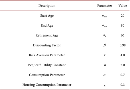
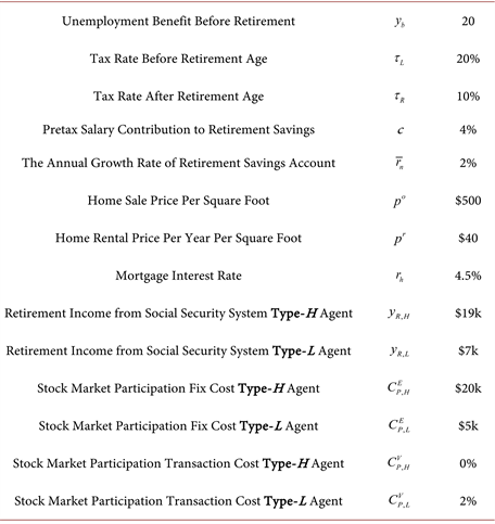
Table 9. Empirical mean vs simulated mean.

Variables

Empirical Mean Value

Simulated Mean Value

Saving Ratio

0.56

0.53

Stock Investment Ratio

0.17

0.17

Liquid Wealth (In thousand dollars)

48.01

67.74

Consumption (In thousand dollars)

35.80

39.61

Stock Investment Amount (In thousand dollars)

29.24

30.06

Bond Investment Amount (In thousand dollars)

44.54

36.80

Participation Ratio

0.45

0.45

Housing Ownership Ratio

0.72

0.75

Figure 6. Goodness of the fit.

4.3. Experiment Results

In order to explore the model’s implication on agent’s behavior. We simulate a large set of $M=20000$ agents through $T=60$ periods, in this simulation, at each period all the agents in the simulated population are of the same age, it is different than the previous simulation which is a cross-generation simulation. Then we study the path of wealth accumulation, stock market participation, home ownership, etc in agents’ life cycles. In such simulations, all agents enter period 0 with $5k initial wealth $w_{-1}$ and zero initial savings in the retirement account $n_{-1}$ . They also enter without owning a home and without any stock market participation experience. Half of the agents $M1=10000$ are Type-H with a high earning profile and easier access to stock investment, the rest half $M2=10000$ is the Type-L with a low earning profile and higher cost when participating the stock investment. ⁹

4.3.1. Simulation Results Overview

In Figure 7, we document the agents’ state changes over their life cycles, and plot the agent’s average portfolio holdings in bonds, stocks, liquid wealth level, retirement savings accounts, etc. The simulation results here can replicate several well-known life-cycle facts. First of all, the average wealth level is hump-shaped for both Type-H and Type-L agents. In Figure 7(a), agents accumulate wealth early on, which peaks in their mid-50s’. Afterward, they finance part of their retirement consumption by gradually decreasing and depleting their liquid wealth. Second, in Figure 7(c), the trajectory of the agent’s non-durable goods consumption trend is smooth as agents dislike violent variation in their marginal utilities over time. The average balance in the retirement saving account increases smoothly and peaks at the time of retirement $a_R=65$ (see Figure 7(f)), and then decreases when agents start to withdraw from the account after retirement.

4.3.2. Type-H Agents vs Type-L Agents

From Figure 7(a), we observe a significant difference in the average liquid wealth level between the two types of agents and the difference becomes even more significant if we combine the liquid wealth with home equity (see Figure 7(b)). Type-H agents can generate around 500k of inheritable wealth at the age of 80 while Type-L agents’ total wealth is negligible. In Figure 7(c) and Figure 7(f), Type-H agents’ average consumption level is much higher and their average 401k balance also outperforms compared with the Type-L agents.

We turn our attention to the portfolio choice of the agents. By default, agents can save through the risk-free bond market. Agents may also choose to access the stock market for high but volatile returns. However, agents need to pay a fixed entry cost upfront and incur variable costs for participating in the stock market. As Figure 7(e) suggests, Type-H agents in the early period of their life cycles, between the age of 23 and the age of 31, choose to invest in the bond market while the wealth level is still low, in order to maintain a smooth consumption level, they are not ready to engage in the risky investment. The increase in wealth level makes them more confident about participating in the stock market. The agents expect a relatively high expected return from the equity market and participate as soon as they reach a comfortable wealth level. In fact for Type-H agents, 27%, 32%, and 20% of them paid the market entry costs at age 30, 31, and 32 respectively (see Figure 7(g)). As indicated in Figure 7(d), Type-H agents place a significant amount of their liquid wealth in the stock market. Around age 35, on average, such agents invest 60k amount of their liquid wealth in the stock market and invest over 80k around age 60. On the other hand, Type-L agents only invest in the bond market, the low earning power and high entry cost, and the lower expected return due to the friction cost drive them away from the stock market. Most of the Type-L agents’ wealth is within the retirement savings.

Figure 7. Simulated mean values of Type-H and Type-L agents.

Housing decision is a byproduct of our model and at the same time influence agents’ investment decision. Figure 7(h) shows the fraction of Type-H agents who own a home at a different point in their life cycle. It is worth noting that almost no agents purchase their homes before the age of 35. There are two forces contributing to this effect. First, as one of the major decisions to make in this environment, agents need to accumulate a sizable down payment in liquid wealth. Second, conditioned on owning a home and carrying forward a mortgage, agents also need to balance the benefit of home ownership versus the potential drop in total wealth in the event of a fire sale, which could be triggered when agents are having liquidity issues and cannot afford the mortgage payment. Thus only when agents who are comfortable with their chances of continuously making payments will become homeowners. It is also shown in Figure 7(h) agents make home purchases between the age of 35 and the age of 45, and eventually, the ownership ratio reaches above 90% around age 50¹⁰. A decline in investment in the stock market between age 35 and age 40 (see Figure 7(d)), is due to the concentrated housing purchase decisions during that age period. Agents do not accumulate much home equity throughout their 20s and only start to do so in their 30s. We believe this replicates the empirical facts well, as reported by Zillow.com, the average age of first-time home-buyer in the US is 34. As shown in Figure 7(h), homeowners hold on to their homes, until the late 70s, when a small fraction of homeowners “fire sale” their homes. Notice the dip in homeownership close to age 80 is a natural result of agents’ winding down their resources toward the end of their life cycle. On the other hand, Type-L agents can only afford to rent the house and do not have the chance to become a homeowner.

4.3.3. Stock Market Decisions from Type-H agents

To understand the factors that drive the stock market decisions, we take a closer look at the simulated Type-H agents population. From Figure 8, we partition the population based on employment status and homeownership status at each age period and compare the aggregated variables between the populations.

As shown by 3 plots from the left column of Figure 8, we observed the unemployment rate stabilizes around 8% over the employable age periods. Employed agents tend to invest significantly more in the stock market and have significantly more liquid wealth on average. This is consistent with our empirical finding that employment is positively correlated with liquid wealth and stock market participation. We believe that the active stock investment for the employed is due to the fact that they are more comfortable about their wealth level, and less worried about their basic consumption needs, given the situation, they can take more risk by participating in the stock market. Participating in the stock market in return generates a higher return on their investment.

From 3 plots on the right column of Figure 8, we observed that fortunate agents accumulate enough wealth and self-selected to become homeowners, this switch in homeownership status happens between age 35 and age 45 then after the age of 50, over 90 % of the agents become homeowners. During this special age period from age 35 to age 50, we observe the change in the investment behavior of agents, starting at the age of 36, while more agents switch from renter to owner, they start to invest more in the stock market, this is also in line with our empirical find that homeowners are more active in stock investment. We believe that home ownership serves as a savings channel for agents to protect them from employment shock and loss in the stock market. Homeownership also exempts agents from paying for housing consumption, letting agents invest more in the stock market. Stock markets on average generate higher returns, homeowners accumulate more liquid wealth than renters as shown in the Figure, and abundant liquid wealth again encourages active stock investment.

Figure 8. Simulated mean values of Type-H Agent population.

4.3.4. Counterfactual Experiments

Through examples of Type-H and Type-L agents, we demonstrate how heterogeneity in earning power and stock market participation cost can potentially cause heterogeneous outcomes in stock market participation, home ownership, and wealth accumulation. Specifically, type-H agents find it easier to participate in the stock market and become homeowners. Type-L agents on the other hand do not have the opportunity to participate in the stock market and can not accumulate enough wealth to make housing purchase.

The assumption we made on both agents is based on the empirical findings that highly educated people tend to have high earning power and at the same time be financially literate. So Type-H agent is different from Type-L agent in both earning power and financial literacy. But to investigate how financial literacy alone could drive this heterogeneous outcome, we conduct the following two counterfactual experiments.

In the first experiment, we ask what happens to Type-H agents’ stock market participation, wealth accumulation, and ownership if they are endowed with stock market participation costs and transaction costs of Type-L agents, we call this new type of agents Type-H-HighCost, indicating the agents have high earning power but are not financially literate. In the second experiment, we ask what happens to Type-L agents’ stock market participation, wealth accumulation, and ownership if they are endowed with participation costs of Type-H, which makes their access to the stock market easier, we call this new type of agents Type-L-LowCost, indicating the agents have low earning power but happen to be financially literate. We conduct the same simulation as shown in 4.3.1 and add the counterfactual experiment results into the existing graph to compare the 4 types of agents: Type-H, Type-L, Type-H-HighCost, Type-L-LowCost at the same time in Figure 9, we applied the same color code to every sub-figure.

From the experiment results shown in Figure 9, if we compare the Type-H-HighCost agents with Type-H agents, we find that the high participation cost decreases the average wealth of Type-H agents (as shown in Figure 9(a)), forces agents to delay home purchasing by 4 years (as shown in Figure 9(e)), forces agents to delay stock participation by more than 10 years, lowers the average consumption level (as shown in Figure 9(b)), significantly decreases the stock investment amount and increases the bond investment amount(as shown in Figure 9(c), Figure 9(d)). On the other hand, if we compare the Type-L-LowCost agents with Type-L agents, easier access to the stock market helps them on average generate more wealth (as shown in Figure 9(a)), slightly elevates their consumption level after the age of 45 (as shown in Figure 9(b)), encourages them to actively participate in the stock investment and even make more investment than Type-H-HighCost agents, becomes less active in bond investment, enables 18% of them to have a chance to become a homeowner, but need to sell the houses due to liquidity needs after retirement (as shown in Figure 9(e)). These results clearly indicate that participation cost alone can play a crucial role in agents’ wealth accumulation, stock market participation, and housing decisions.

Finally, we want to put ourselves in the perspective of the Type-L agents, given that Type-L agents are not financially literate, there is still a chance for them to participate in stock investment. We ran another experiment on the Type-L agents by slightly making the agents less risk-averse and more patient in consumption. We achieve this by decreasing the risk-aversion parameter value to $\gamma =3.0$ and increasing the discounting factor value to $\beta =0.99$ in Table 8, we could still generate a stock market participation ratio of around 12%.

Figure 9. Simulated mean values.

5. Conclusion

We are motivated by the empirical findings that there exists a positive correlation between labor market skill and stock market participation, and we build a life-cycle model to assess the role played by financial literacy in wealth accumulation. More specifically, we consider the portfolio choice problem in an environment with labor income risks, housing consumption, and retirement savings. Our model shows a good fit in the empirical portfolio choice, homeownership, and consumption pattern. We conclude that both high-earning power and financial literacy encourage agents’ stock market participation in the early period of their life cycle and active stock market investment in turn helps with wealth accumulation.

As to the “participation puzzle”, when approximated by a fixed entry cost and variable costs, our findings support that stock market participation plays a crucial role in generating heterogeneous outcomes in agents’ wealth accumulation, increasing wealth inequality. In lieu of financial innovation such as Robinhood and other investment platforms, this finding would provide policy-makers support in promoting financial innovation that would level the playing field by reducing the market entry cost. Some recent studies have shown evidence of the advantage of low-cost investment platforms: Barber et al. (2022) , Welch (2022) . We also further conjecture that low-cost investment platforms, when properly guided, have the potential to address social inequality issues through increasing stock market participation.

However, there are several shortcomings in our current life-cycle model. First of all, the relative price of housing and rental units are assumed to be constant, so there is no capital gain from home ownership. Thus, home ownership is primarily a savings channel. A more realistic model of housing price dynamics would help generate a better fit for the current model. Second, we build the model in the traditional fully rational expectation framework (Skinner, 2007; Attanasio & Weber, 2010) . However, empirical evidence points towards a reality where households are not perfectly rational when it comes to financial decisions. We can alternatively, introduce elements of behavioral economics, where agents’ policy function does not necessarily come from “backward induction”. For example, as in Choi et al. (2009) , investors increase their investment in their 401k account when they experience higher and steadier returns in the previous years. We would then compare the policies of behavior agents to those of the fully rational agents, and assess each model’s ability to match empirical patterns in household finance. Finally, driven by technological advancements and increasing competition among financial service providers, the trend of lowering fees and charges for stock market investment has been ongoing for several years. We could potentially shift our focus from modeling the heterogeneity of participation cost to the heterogeneity of agents’ ability to predict the market, although we think these heterogeneities are all driven by the heterogeneity in financial literacy.

Acknowledgements

The authors wish to thank Mark Paddrik, Anand Goel, Mai Feng, Zakaria Babutsidze and conference participants at the WEAI, EEA, International Finance and Banking Society for useful comments and suggestions, any errors are ours.

Appendices

Additional Summary Statistics

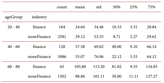
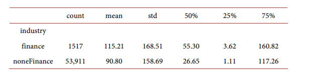
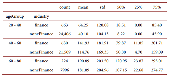
Stock investment amount conditioning on participation for households with and without finance industry experience:

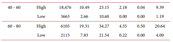
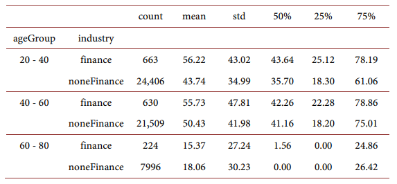
For different household head age groups:

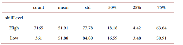
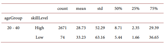
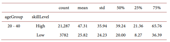
Stock investment amount conditioning on participation for high-skilled household and low-skilled households:

For different household age groups:

Liquid wealth for household with and without finance industry experience:

For different household age groups:

Liquid wealth for high-skilled household and low-skilled households:

For different household age groups:

Labor income for household with and without finance industry experience:

For different household age groups:

Labor income for high-skilled household and low-skilled households:

For different household age groups:

Total wealth with home equity for household with and without finance industry experience:

For different household age groups:

Total wealth for high-skilled household and low-skilled households:

For different household age groups:

NOTES

¹The problem, called the “equity premium puzzle”, was first publicized by Mehra and Prescott (1985), and it is described as that observed rates of return on equity are “excessive”, i.e. they are much higher than it is predicted by the theory based on general equilibrium models.

²By financial literacy, the current draft refers to the ability to access the stock market. However, a broader definition of literacy exists. From a modeling perspective, “understanding compounding” gives you a higher propensity to save, and “understanding risk diversification” gives you a higher propensity to buy your home. The survey also shows that homeowners tend to be more financially literate than non-home-owners.

³PSID is a publicly available longitudinal household survey data set that began in 1968 with a nationally representative sample of over 18,000 individuals living in 5,000 families in the United States. The PSID is directed by faculty at the University of Michigan.

⁴The choice of the year of dollar value is arbitrary, and different choices of the year would have an immaterial impact on the observed trend in the data.

⁵Recall the ordinary annuity formula, such that $PV=PMT\cdot \frac{1-\frac{1}{{\left(1+\bar{r}\right)}^{N_t}}}{\bar{r}}$ .

⁶Survey shows that home-ownership rate is higher amongst the financially literate population. It is argued by people like Shiller that, real-estate investment, even if taking into consideration of leverage, do not outperform stock investment historically in the last 120 years or so. We, therefore, think of home ownership as a form of durable consumption that yields higher utility than renting unconditionally. When it comes to a home-ownership decision, we assume that financially literate people do not outperform non-literate people financially. This modeling strategy generates results that are consistent with empirical observation where literate people are more likely to own homes.

⁷A more detailed view of the income processes for two types of agents is shown in Figure 2.

⁸The Survey of Consumer Finances (SCF) is a triennial survey conducted by the Federal Reserve Board in the United States. The survey collects detailed information on the finances of U.S. households, including their income, assets, debts, and financial behaviors.

⁹Alternatively, one can simulate M_e economies each with a unique path of aggregate state ${\left\{S_t\right\}}_{t=1}^T$ . For each economy m, one can then generate a large number of agents to track their actions in their life cycles.

¹⁰Notice since all mortgages have a 30-year term and the agents, live up to 80, age 49 is the last period in which the renter can become a home-owner.

Conflicts of Interest

The authors declare no conflicts of interest regarding the publication of this paper.

References

[1]	Alan, S. (2006). Entry Costs and Stock Market Participation over the Life Cycle. Review of Economic Dynamics, 9, 588-611. https://doi.org/10.1016/j.red.2006.06.003
[2]	Arellano, M., Blundell, R., & Bonhomme, S. (2017). Earnings and Consumption Dynamics: A Nonlinear Panel Data Framework. Econometrica, 85, 693-734. https://doi.org/10.3982/ECTA13795
[3]	Athreya, K. B., Ionescu, F., & Neelakantan, U. (2015). Stock Market Investment: The Role of Human Capital. Finance and Economics Discussion Series 2015-65. Board of Governors of the Federal Reserve System (U.S.). https://ideas.repec.org/p/fip/fedgfe/2015-65.html
[4]	Attanasio, O. P., & Weber, G. (2010). Consumption and Saving: Models of Intertemporal Allocation and Their Implications for Public Policy. Journal of Economic Literature, 48, 693-751. https://doi.org/10.1257/jel.48.3.693
[5]	Barber, B. M., Huang, X., Odean, T., & Schwarz, C. (2022). Attention-Induced Trading and Returns: Evidence from Robinhood Users. The Journal of Finance, 77, 3141-3190. https://doi.org/10.1111/jofi.13183
[6]	Ben-Porath, Y. (1967). The Production of Human Capital and the Life Cycle of Earnings. Journal of Political Economy, 75, 352-365. http://www.jstor.org/stable/1828596 https://doi.org/10.1086/259291
[7]	Bernheim, B., & Garrett, D. M. (2003). The Effects of Financial Education in the Workplace: Evidence from a Survey of Households. Journal of Public Economics, 87, 1487-1519. https://www.sciencedirect.com/science/article/pii/S0047272701001840
[8]	Cagetti, M. (2003). Wealth Accumulation over the Life Cycle and Precautionary Savings. Journal of Business & Economic Statistics, 21, 339-353. https://doi.org/10.1198/073500103288619007
[9]	Choi, J. J., Laibson, D., Madrian, B. C., & Metrick, A. (2009). Reinforcement Learning and Savings Behavior. The Journal of Finance, 64, 2515-2534. https://doi.org/10.1111/j.1540-6261.2009.01509.x
[10]	Delavande, A., Rohwedder, S., & Willis, R. (2008). Preparation for Retirement, Financial Literacy and Cognitive Resources. Michigan Retirement Research Center Research Paper. https://econpapers.repec.org/repec:mrr:papers:wp190
[11]	Fisher, I. (1930). Theory of Interest: As Determined by Impatience to Spend Income and Opportunity to Invest It. Augustusm Kelly Publishers.
[12]	Gomes, F., & Michaelides, A. (2005). Optimal Life-Cycle Asset Allocation: Understanding the Empirical Evidence. The Journal of Finance, 60, 869-904. https://doi.org/10.1111/j.1540-6261.2005.00749.x
[13]	Guvenen, F. (2009). A Parsimonious Macroeconomic Model for Asset Pricing. Econometrica, 77, 1711-1750. https://doi.org/10.3982/ECTA6658
[14]	Hong, H., Kubik, J. D., & Stein, J. C. (2004). Social Interaction and Stock-Market Participation. Journal of Finance, 59, 137-163. https://doi.org/10.1111/j.1540-6261.2004.00629.x
[15]	Huggett, M., Ventura, G., & Yaron, A. (2011). Sources of Lifetime Inequality. American Economic Review, 101, 2923-54. https://doi.org/10.1257/aer.101.7.2923
[16]	Jagannathan, R., Kocherlakota, N. R. et al. (1996). Why Should Older People Invest Less in Stocks than Younger People. Federal Reserve Bank of Minneapolis Quarterly Review, 20, 11-20. https://doi.org/10.21034/qr.2032
[17]	Mehra, R., & Prescott, E. C. (1985). The Equity Premium: A Puzzle. Journal of Monetary Economics, 15, 145-161. https://doi.org/10.1016/0304-3932(85)90061-3
[18]	Skinner, J. (2007). Are You Sure You’re Saving Enough for Retirement? Journal of Economic Perspectives, 21, 59-80. https://doi.org/10.1257/jep.21.3.59
[19]	van Rooij, M., Lusardi, A., & Alessie, R. (2011). Financial Literacy and Stock Market Participation. Journal of Financial Economics, 101, 449-472. https://www.sciencedirect.com/science/article/pii/S0304405X11000717
[20]	Vestman, R. (2019). Limited Stock Market Participation among Renters and Homeowners. The Review of Financial Studies, 32, 1494-1535. https://doi.org/10.1093/rfs/hhy089
[21]	Welch, I. (2022). The Wisdom of the Robinhood Crowd. The Journal of Finance, 77, 1489-1527. https://doi.org/10.1111/jofi.13128
[22]	Wong, A. (2015). Population Aging and the Transmission of Monetary Policy to Consumption. Job Market Paper, Northwestern University.
[23]	Xie, M. (2021). Family Wealth Accumulation and Fiscal Prudence among China’s Young Adults: Between the Privileged and the Common. Open Journal of Social Sciences, 9, 478-498. https://doi.org/10.4236/jss.2021.99035
[24]	Zhu, H. (2019). The Impact of Home Equity and Housing Provident Fund on the Household’s Stock Investment. Open Journal of Social Sciences, 7, 222-240. https://doi.org/10.4236/jss.2019.78016