The Modified BAPG_s Method for Support Vector Machine Classifier with Truncated Loss

Kexin Ren

School of Information Science and Technology, Jinan University, Guangzhou, China.

DOI: 10.4236/am.2024.154015                

Abstract

In this paper, we modify the Bregman APG_s (BAPG_s) method proposed in (Wang, L, et al.) for solving the support vector machine problem with truncated loss (HTPSVM) given in (Zhu, W, et al.), we also add an adaptive parameter selection technique based on (Ren, K, et al.). In each iteration, we use the linear approximation method to get the explicit solution of the subproblem and set a function to apply the Bregman distance. Finally, numerical experiments are performed to verify the efficiency of BAPG_s.

Keywords

HTPSVM, Bregman Distance, BAPG_s Algorithm

1. Introduction

SVM (Support Vector Machine) [1] is a supervised learning algorithm commonly used for classification tasks and has been successfully applied to many technological fields, such as text categorization [2] , financial forecast [3] , image classification [4] and so on. This paper focuses on a binary classification problem. Given training samples $\left\{\left(x_i,y_i\right),i=1,\cdots ,m\right\}$ , where $x_i\in {ℝ}^n$ , $y_i\in \left\{-\mathrm{1,1}\right\}$ , the objective of SVM is to identify an optimal separating hyperplane to separate data points into two classes. Scholars have proposed some classic SVM models based on convex loss functions, such as the hinge loss (also called L₁ loss) in classic SVM [5] , the least square loss in LSSVM [6] and the huberized pinball loss in HPSVM [7] . However, in practice, the real dataset often contain noise. Since convex loss functions are generally unbounded, convex losses are highly sensitive to outliers and potentially influenced by outliers. Therefore, some nonconvex loss functions are proposed to improve robustness compared with the convex loss functions [8] . For example, [9] proposed the ramp loss based on hinge loss, the truncated pinball loss was proposed by [10] . Recently, a noise insensitive and robust support vector machine classifier with huberied truncated pinball loss (HTPSVM) was proposed in [11] , this loss is smooth and nonconvex loss function. The HTPSVM can be transformed into format of “Loss + Penalty”, in which the penalty is a hybrid of $l_1$ norm and $l_2$ norm penalty.

Here, the HTPSVM model and algorithm of literature [11] are briefly introduced. Consider a classification problem with training samples ${\left\{x_i\mathrm{,}{y}_i\right\}}_{i=1}^m\subset {ℝ}^d\times \left\{-\mathrm{1,1}\right\}$ . The HTPSVM seeks to solve the following regularization problem:

$\underset{b\in ℝ,w\in {ℝ}^d}{\min }\frac{1}{m}{\displaystyle \underset{i=1}{\overset{m}{\sum }}}{\mathcal{l}}_{htp}\left(y_i\left(b+w^{\text{T}}{x}_i\right)\right)+\lambda {\Vert w\Vert }_1+\frac{{\Vert w\Vert }_2^2}{2}+\frac{b^2}{2},$ (1)

the huberied truncated pinball loss ${\mathcal{l}}_{htp}(\cdot )$ function is defines as

${\mathcal{l}}_{htp}\left(u\right)=\{\begin{array}{ll}1,\hfill & u\le -\frac{2}{5}\hfill \\ \frac{4}{5}-u-\frac{5}{4}{u}^2,\hfill & -\frac{2}{5}<u\le 0,\hfill \\ \frac{4}{5}-u,\hfill & 0<u\le \frac{3}{5},\hfill \\ \frac{5}{4}{\left(1-u\right)}^2,\hfill & \frac{3}{5}<u\le 1,\hfill \\ \frac{5}{8}{\left(1-u\right)}^2,\hfill & 1\le u<\frac{7}{5},\hfill \\ -\frac{1}{2}\left(\frac{6}{5}-u\right),\hfill & \frac{7}{5}\le u<\frac{8}{5},\hfill \\ -\frac{1}{2}\left(\frac{6}{5}-u\right)-\frac{5}{8}{\left(u-\frac{8}{5}\right)}^2,\hfill & \frac{8}{5}\le u<2,\hfill \\ \frac{3}{10},\hfill & u\ge 2,\hfill \end{array}$ (2)

which is a nonconvex and smooth function. The HTPSVM combine the benefits of both $l_1$ and $l_2$ norm regularizers and and it has been demonstrated in [11] that it can reduce the effects of noise in the training sample. Therefore, we consider that studying the HTPSVM model is meaningful. The APG algorithm was used to solve the model in [11] . [12] applied the APG_s method (first proposed in [13] ) to solve problem (1) and obtain better convergence behavior. However we find that the proximal operator for computing the $l_1$ norm causes the subproblem to be solved slowly in APG and APG_s algorithms, we attempt to accelerate the solution process for this model. Recently, [14] propose the Bregman APG_s (BAPG_s) method, which avoids the restrictive global Lipschitz gradient continuity assumption. In this paper, we improve BAPG_s algorithm to solve the problem (1) and replace the Lipschitz constant by an appropriate positive definite matrix and obtain better results after we perform numerical experiments on 10 datasets to test our method.

The rest of this paper is organized as follows. In the next section, we provide preliminary materials used in this work. In Section 3, we introduce the BAPG_s algorithm proposed by [14] and present our algorithm based on the BAPG_s method for solving the HTPSVM model (1). The convergence of our method is also discussed. Section 4 performs some experiments.

2. Preliminaries

In this paper, we let $ℝ$ denote the set of real numbers. We work in the Euclidean space ${ℝ}^n$ , and the standard Euclidean inner product and the induced norm on ${ℝ}^n$ are denoted by $\langle \cdot \mathrm{,}\cdot \rangle$ and $\Vert \cdot \Vert$ . The domain of the function $f\mathrm{<mo>\; :\; </mo>}{ℝ}^n\to \left(-\infty \mathrm{,}+\infty \right]$ is defined by $\text{dom}f=\left\{x\in {ℝ}^n:f\left(x\right)<+\infty \right\}$ . We say that f is proper if $\text{dom}f\ne \varnothing$ . A proper function f is said to be closed if it is lower semicontinuous at any $x\in \text{dom}f$ , i.e. $f\left(x\right)\le \lim {\inf }_{z\to x}f\left(z\right)$ .

Definition 1. [ [15] , Definition 8.3] For a proper closed function f, the regular subdifferential of $f\mathrm{<mo>\; :\; </mo>}{ℝ}^n\to ℝ\cup \left\{+\infty \right\}$ at $x\in \text{dom}f$ is defined by

$\hat{\partial }f\left(x\right):=\left\{\hat{x}\in {ℝ}_n:\underset{z\to x,z\ne x}{\lim \inf }\frac{f\left(z\right)-f\left(x\right)-\langle \hat{x},z-x\rangle }{\Vert z-x\Vert }\ge 0\right\}.$ (3)

The (general) subdifferential of f at $x\in \text{dom}f$ is defined

$\partial f\left(x\right)\mathrm{<mo>\; :\; </mo>}=\left\{\hat{x}\mathrm{<mo>\; :\; </mo>}\exists x^k\stackrel{f}{\to }x\mathrm{,}{\hat{x}}^k\to \hat{x}\text{with}{\hat{x}}^k\in \hat{\partial }f\left(x^k\right)\text{for}\text{each}k\right\}\mathrm{,}$ (4)

where $x^k\stackrel{f}{\to }x$ means both $x^k\to x$ and $f\left(x^k\right)\to f\left(x\right)$ . Note that if f is also convex, then the general subdifferential and regular subdifferential of f at $x\in \text{dom}f$ reduce to the classical subdifferential [ [15] , Proposition 8.12], that is $\partial f\left(x\right)=\left\{\hat{x}\mathrm{<mo>\; :\; </mo>}f\left(y\right)\ge f\left(x\right)+\langle \hat{x}\mathrm{,}y-x\rangle \text{for}\text{all}y\right\}\mathrm{.}$ (5)

Definition 2. (Kernel Generating Distances and Bregman Distances [16] [17] [18] ) Let C be a nonempty, convex and open subset of ${ℝ}^n$ . Associated with C, a function $\varphi \mathrm{<mo>\; :\; </mo>}{ℝ}^n\to \left(-\infty \mathrm{,}+\infty \right]$ is called a kernel generating distance if it satisfies the following:

1) $\varphi$ is proper, lower semicontinuous and convex, with $\text{dom}\varphi \subset \bar{C}$ and $\text{dom}\partial \varphi =C$ ;

2) $\varphi$ is continuously differentiable on $\mathrm{int}\text{dom}\varphi \equiv C$ .

We denote the class of kernel generating distances by $\mathcal{G}\left(C\right)$ . Given $\varphi \in \mathcal{G}\left(C\right)$ , the Bregman distance $D_{\varphi }:\text{dom}\varphi \times \mathrm{int}\text{dom}\varphi \to \left(0,+\infty \right]$ is defined by

$D_{\varphi }\left(x\mathrm{,}y\right)\mathrm{<mo>\; :\; </mo>}=\varphi \left(x\right)-\varphi \left(y\right)-\langle \nabla \varphi \left(y\right)\mathrm{,}x-y\rangle \mathrm{.}$

For exmple, when $\varphi \left(x\right)={\Vert x\Vert }^2$ , then $D_{\varphi }\left(x\mathrm{,}y\right)={\Vert x-y\Vert }^2$ . If $\varphi \left(x\right)=x^{\text{T}}Ax$ , then $D_{\varphi }\left(x\mathrm{,}y\right)={\left(x-y\right)}^{\text{T}}A\left(x-y\right)$ . In this article, the gradient Lipschitz continuity condition of the function f is no longer required, instead it is replaced by the L-smooth adaptive function of pair $\left(f\mathrm{,}\varphi \right)$ . The definition of L-smooth adaptable as follows.

Definition 3. A pair of functions $\left(f\mathrm{,}\varphi \right)$ , $\varphi \in \mathcal{G}\left(C\right)$ , $f\mathrm{<mo>\; :\; </mo>}{ℝ}^n\to \left(-\infty \mathrm{,}+\infty \right]$ is a proper and lower semicontinuous function with $\text{dom}\varphi \subset \text{dom}f$ and f is continuously differentiable on $C=\mathrm{int}\text{dom}\varphi$ , is called L-smooth adaptable (L-smad) on C if there exists $L>0$ such that $L\varphi -f$ and $L\varphi +f$ are convex on C.

Lemma 1. (Full Extended Descent Lemma [19] ) A pair of functions $\left(f\mathrm{,}\varphi \right)$ is L-smad on $C=\mathrm{int}\text{dom}\varphi$ if and only if: $\left|f\left(x\right)-f\left(y\right)-\langle \nabla f\left(y\right),x-y\rangle \right|\le L{D}_{\varphi }\left(x,y\right)$ , $\forall x,y\in \mathrm{int}\text{dom}\varphi$ .

Definition 4. $f\mathrm{<mo>\; :\; </mo>}{ℝ}^n\to ℝ\cup \left\{+\infty \right\}$ is called μ-relative weakly convex to $\varphi$ on C if there exists $\mu >0$ such that $f+\mu \varphi$ is convex on C [14] .

3. The Modified BAPG_s Method for HTPSVM

In this section, we first describe the BAPG_s method proposed in [14] , then the modified BAPG_s method with adaptive parameter is given for HTPSVM.

3.1. BAPG_s Method

Consider the following optimization problem:

$\underset{x\in {ℝ}^n}{\min }F\left(x\right)\mathrm{<mo>\; :\; </mo>}=f\left(x\right)+P_1\left(x\right)-P_2\left(x\right)\mathrm{,}$ (6)

where f is a μ-relative weakly convex continuously differentiable function, P₁ is a proper, lower semicontinuous convex function and P₂ is continuous and convex. Besides, F is level-bounded i.e., for every $\alpha \in ℝ$ , the set $\left\{x\in {ℝ}^n|F\left(x\right)\le \alpha \right\}$ is bounded; F is bounded below i.e., ${\inf }_{x\in {ℝ}^n}F\left(x\right)>-\infty$ . The iterative scheme of BAPG_s [14] for solving probelm (6) is shown in Algorithm 1, where $D_{\varphi }$ is a Bregman distance defined in Section 2.

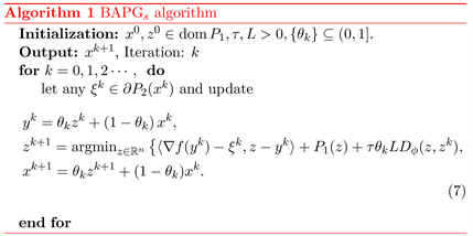
We see that when $D_{\varphi }\left(x\mathrm{,}y\right)=\frac{1}{2}{\Vert x-y\Vert }^2$ , BAPG_s reduces to APG_s in [13] . [14] proved the global convergence of the iterates generated by BAPG_s to a limiting critical point under some assumptions.

3.2. Adaptive BAPG_s Method for HTPSVM

By writing the nonconvex loss ${\mathcal{l}}_{htp}$ as the difference of three smooth convex functions, the problem (1) can be expressed as following from [12]

$\underset{b\in ℝ,w\in {ℝ}^d}{\min }F\left(b\mathrm{,}w\right)=f_1\left(b\mathrm{,}w\right)-f_2\left(b\mathrm{,}w\right)-f_3\left(b\mathrm{,}w\right)+P_1\left(b\mathrm{,}w\right)\mathrm{,}$ (8)

where $P_1\left(b\mathrm{,}w\right)=\lambda {\Vert w\Vert }_1+\frac{{\Vert w\Vert }_2^2}{2}+\frac{b^2}{2}$ , $\lambda$ is the regularization parameter; for $j=\mathrm{1,2}$ , $f_j\left(b,w\right)=\frac{1}{m}{\displaystyle {\sum }_{i=1}^m}{\mathcal{l}}_j\left[y_i\left(b+w^{\text{T}}{x}_i\right)\right]$ , and the smooth convex functions ${\mathcal{l}}_j$ are defined as

${\mathcal{l}}_1\left(u\right)=\{\begin{array}{lll}\frac{4}{5}-u\mathrm{,}\hfill & \text{if}\hfill & u<\frac{3}{5},\hfill \\ \frac{5}{4}{\left(1-u\right)}^2\mathrm{,}\hfill & \text{if}\hfill & \frac{3}{5}\le u<1,\hfill \\ \frac{5}{8}{\left(1-u\right)}^2\mathrm{,}\hfill & \text{if}\hfill & 1\le u<\frac{7}{5},\hfill \\ -\frac{1}{2}\left(\frac{6}{5}-u\right)\mathrm{,}\hfill & \text{if}\hfill & u\ge \frac{7}{5}\mathrm{,}\hfill \end{array}$ (9)

${\mathcal{l}}_2\left(u\right)=\{\begin{array}{lll}-u-\frac{1}{5}\mathrm{,}\hfill & \text{if}\hfill & u\le -\frac{2}{5}\mathrm{,}\hfill \\ \frac{5}{4}{u}^2\mathrm{,}\hfill & \text{if}\hfill & -\frac{2}{5}<u\le 0,\hfill \\ \mathrm{0,}\hfill & \text{if}\hfill & u\ge \mathrm{0,}\hfill \end{array}$ (10)

${\mathcal{l}}_3\left(u\right)=\{\begin{array}{lll}\mathrm{0,}\hfill & \text{if}\hfill & u\le \frac{8}{5}\mathrm{,}\hfill \\ \frac{5}{8}{\left(u-\frac{8}{5}\right)}^2\mathrm{,}\hfill & \text{if}\hfill & \frac{8}{5}\le u<2,\hfill \\ -\frac{1}{2}\left(\frac{9}{5}-u\right)\mathrm{,}\hfill & \text{if}\hfill & u\ge 2.\hfill \end{array}$ (11)

Then we can apply the BAPG_s to solve problem (8) in the form of (6)

• ${\mathcal{P}}_1$ : $f=f_1-f_3$ (nonconvex), $P_2=f_2$ (convex);

• ${\mathcal{P}}_2$ : $f=f_1-f_2$ (nonconvex), $P_2=f_3$ (convex).

Next, We will briefly illistrate that the problem (8) can be solved by the BAPG_s [14] .

Theorem 1. Let f as defined in ${\mathcal{P}}_1$ and ${\mathcal{P}}_2$ . Set $\varphi \left(x\right)\mathrm{<mo>\; :\; </mo>}=\frac{1}{2}{x}^{\text{T}}Qx$ , where $Q=\frac{1}{m}{\displaystyle {\sum }_{i=1}^m}\frac{5}{2}{Q}_i$ , $Q_i={\left(y_i\mathrm{,}{y}_i{x}_i^{\text{T}}\right)}^{\text{T}}\left(y_i\mathrm{,}{y}_i{x}_i^{\text{T}}\right)$ . Then, the pair $\left(f\mathrm{,}\varphi \right)$ is L-smooth adaptable on ${ℝ}^n$ with $L=1$ .

Proof. Firstly, for ${\mathcal{P}}_1$ , since

${{\mathcal{l}}^{\prime }}_{1-3}\left(u\right)+\frac{5}{2}u=\{\begin{array}{lll}\frac{5}{2}u-1,\hfill & \hfill & u\le \frac{3}{5},\hfill \\ 5u-\frac{5}{2},\hfill & \hfill & \frac{3}{5}<u\le 1,\hfill \\ \frac{15}{4}u-\frac{5}{4},\hfill & \hfill & 1\le u<\frac{7}{5},\hfill \\ \frac{5}{2}u+\frac{1}{2},\hfill & \hfill & \frac{7}{5}\le u<\frac{8}{5},\hfill \\ \frac{5}{4}u+\frac{5}{2},\hfill & \hfill & \frac{8}{5}\le u<2,\hfill \\ \frac{5}{2}u,\hfill & \hfill & u\ge 2,\hfill \end{array}$ (12)

and

$\frac{5}{2}u-{{\mathcal{l}}^{\prime }}_{1-3}\left(u\right)=\{\begin{array}{lll}\frac{5}{2}u+1,\hfill & \hfill & u\le \frac{3}{5},\hfill \\ \frac{5}{2},\hfill & \hfill & \frac{3}{5}<u\le 1,\hfill \\ \frac{5}{4}u+\frac{5}{4},\hfill & \hfill & 1<u\le \frac{7}{5},\hfill \\ \frac{5}{2}u-\frac{1}{2},\hfill & \hfill & \frac{7}{5}\le u<\frac{8}{5},\hfill \\ \frac{15}{4}u-\frac{5}{2},\hfill & \hfill & \frac{8}{5}\le u<2,\hfill \\ \frac{5}{2}u,\hfill & \hfill & u\ge 2,\hfill \end{array}$ (13)

are monotonically increasing, it is easy to verify that ${\mathcal{l}}_{1-3}\left(u\right)+\frac{5}{4}{u}^2$ and $\frac{5}{4}{u}^2-{\mathcal{l}}_{1-3}\left(u\right)$ are convex. Then we can easily get the convexity of

$\begin{array}{c}f\left(b,w\right)+\frac{1}{2}{x}^{\text{T}}Qx=\frac{1}{m}{\displaystyle \underset{i=1}{\overset{m}{\sum }}}{\mathcal{l}}_{1-3}\left[y_i\left(b+w^{\text{T}}{x}_i\right)\right]+\frac{1}{2m}{\displaystyle \underset{i=1}{\overset{m}{\sum }}}\frac{5}{2}{\left(b;w\right)}^{\text{T}}{Q}_i\left(b;w\right)\\ =\frac{1}{m}{\displaystyle \underset{i=1}{\overset{m}{\sum }}}\left[{\mathcal{l}}_{1-3}\left[y_i\left(b+w^{\text{T}}{x}_i\right)\right]+\frac{5}{4}{\left(b;w\right)}^{\text{T}}{Q}_i\left(b;w\right)\right]\\ =\frac{1}{m}{\displaystyle \underset{i=1}{\overset{m}{\sum }}}\left[{\mathcal{l}}_{1-3}\left[y_i\left(b+w^{\text{T}}{x}_i\right)\right]+\frac{5}{4}{\left[y_i\left(b+w^{\text{T}}{x}_i\right)\right]}^2\right],\end{array}$ (14)

and

$\frac{1}{2}{x}^{\text{T}}Qx-f\left(b,w\right)=\frac{1}{m}{\displaystyle \underset{i=1}{\overset{m}{\sum }}}\left[\frac{5}{4}{\left[y_i\left(b+w^{\text{T}}{x}_i\right)\right]}^2-{\mathcal{l}}_{1-3}\left[y_i\left(b+w^{\text{T}}{x}_i\right)\right]\right],$ (15)

the proof is similar for ${\mathcal{P}}_2$ . It is clear that $\left(f\mathrm{,}\varphi \right)$ is 1-smooth adaptable on ${ℝ}^n$ , this further implies that there exists $0<\mu \le 1$ such that $f+\mu \varphi$ is convex.

We can see that the problem (8) satisfies the conditions required in [14] with $\varphi \left(x\right)=\frac{1}{2}{x}^{\text{T}}Qx$ for the pair $\left(f\mathrm{,}\varphi \right)$ , where Q defined as Theorem 1. Therefore the BAPG_s method (Algorithm 1), here we let $\tau =1$ and replace (7) with the following steps, can be used for solving (8)

$\begin{array}{l}{y}^k={\theta }_k{z}^k+\left(1-{\theta }_k\right)x^k,\\ z^{k+1}=\arg {\min }_{z\in {ℝ}^n}\left\{\langle \nabla f\left(y^k\right)-{\xi }^k,z-y^k\rangle +P_1\left(z\right)+\frac{{\theta }_k}{2}\left[{\left(z-z^k\right)}^{\text{T}}Q\left(z-z^k\right)\right]\right\},\\ x^{k+1}={\theta }_k{z}^{k+1}+\left(1-{\theta }_k\right)x^k.\end{array}$ (16)

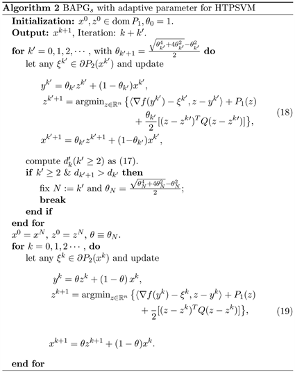
The selection of parameter $\left\{{\theta }_k\right\}$ in [14] as: for fixed positive integer N, let ${\theta }_0=1$ ,

${\theta }_{k+1}=\frac{\sqrt{{\theta }_k^4+4{\theta }_k^2}-{\theta }_k^2}{2}\mathrm{,}k=\mathrm{1,2,}\cdots \mathrm{,}N$

and ${\theta }_k\equiv {\theta }_N$ for all $k>N$ . It is to see that the value of the positive integer N is difficult to determine. Combining with the adaptive parameter selection criterion proposed in [12] : let ${\theta }_0=1$ , ${\theta }_k=\frac{\sqrt{{\theta }_{k-1}^4+4{\theta }_{k-1}^2}-{\theta }_{k-1}^2}{2}$ for $k\ge 1$ and compute

$d_k\mathrm{<mo>\; :\; </mo>}=\frac{H_{k-1}-H_k}{{\left(x^k-x^{k-1}\right)}^{\text{T}}\left(x^k-x^{k-1}\right)}\mathrm{,}$ (17)

when $k\ge 2$ , where $H_k\mathrm{<mo>\; :\; </mo>}=F\left(x^k\right)+\frac{{\beta }_k}{2}{\left(x^k-x^{k-1}\right)}^{\text{T}}Q\left(x^k-x^{k-1}\right)$ and ${\beta }_k=\frac{{\alpha }_k}{{\theta }_{k-1}^2}$ (the assumption of sequence $\left\{{\alpha }_k\right\}$ given in [14, Assumption 2]). Let N be the first k satisfying $d_k\le d_{k+1}$ . The BAPG_s algorithm with adaptive parameter for problem (8) (HTPSVM) is shown in Algorithm 2.

4. Numerical Results

In this section, we aim to show the performance of Algorithm 2 for solving problem (1) by using MATLAB R2020b on a 64-bit PC with an Intel(R) Core(TM) i7-10870H CPU (2.20GHz) and 16GB of RAM.

First, consider the optimality condition (19) of Algorithm 2

$\begin{array}{c}0\in \nabla f\left(y^{k^{\prime }}\right)-{\xi }^k+\partial P_1\left(z^{k+1}\right)+\theta Q\left(z^{k+1}-z^k\right)\\ =\nabla f\left(y^k\right)-{\xi }^k+\lambda \partial {\Vert z^{k+1}\Vert }_1+z^{k+1}+\theta Q\left(z^{k+1}-z^k\right)\mathrm{.}\end{array}$

Due to there is no explicit solution for this subproblem, we try to instead the $l_1$ norm by linear approximation, that is, ${\Vert z\Vert }_1\approx {\Vert x^k\Vert }_1+v^k{}^{{}^{\text{T}}}\left(z-x^k\right)$ , where $v^k\in \partial {\Vert x^k\Vert }_1$ (here we take $v^k\mathrm{<mo>\; :\; </mo>}=\text{sign}\left(x^k\right)$ ), then we construct a new iteration step to replace the subproblem in Algorithm 2 as

$\begin{array}{c}{z}^{k+1}=\arg {\min }_{z\in {ℝ}^n}\{\langle \nabla f\left(y^k\right)-{\xi }^k,z-y^k\rangle +{\Vert x^k\Vert }_1+\lambda v^k{}^{{}^{\text{T}}}\left(z-x^k\right)\stackrel{}{}\\ +\frac{1}{2}{z}^{\text{T}}z+\frac{\theta }{2}\left[{\left(z-z^k\right)}^{\text{T}}Q\left(z-z^k\right)\right]\},\end{array}$ (20)

it is easy to calculate its solution:

$0=\nabla f\left(y^k\right)-{\xi }^k+\lambda v^k{}^{{}^{\text{T}}}+z^{k+1}+\theta Q\left(z^{k+1}-z^k\right)\mathrm{,}$

which means

$\left(I+\theta Q\right)z^{k+1}=\theta Q{z}^k-\nabla f\left(y^k\right)+{\xi }^k-\lambda v^k\mathrm{.}$

Then the update (18) and (19) are replaced by

$\{\begin{array}{l}{z}^{k^{\prime }+1}={\left(I+{\theta }_{k^{\prime }}Q\right)}^{-1}\left({\theta }_{k^{\prime }}Q{z}^{k^{\prime }}-\nabla f\left(y^{k^{\prime }}\right)+{\xi }^{k^{\prime }}-\lambda v^{k^{\prime }}\right)\mathrm{,}\hfill \\ z^{k+1}={\left(I+\theta Q\right)}^{-1}\left(\theta Q{z}^k-\nabla f\left(y^k\right)+{\xi }^k-\lambda v^k\right)\mathrm{,}\hfill \end{array}$ (21)

in experiments, where $v^{k^{\prime }}=\text{sign}\left(x^{k^{\prime }}\right)$ and $v^k=\text{sign}\left(x^k\right)$ . The experiments are conducted on several real world datasets. We select 10 datasets from UCI [20] , to compare the Algorithm 2 with APG (method in [11] ), APG_s [12] and GIST [21] , where in GIST, we set $F=f+P_1$ with $f=f_1-f_2-f_3$ . The corresponding parameters of these methods are set the same as in [12] . For each dataset, The 21 initial points are used commonly for all methods: one zero vector, and 5 vectors selected independently from N (0, σ²I) for each $\sigma \in \left\{\mathrm{1,2,4,8}\right\}$ . All algorithms stop if $\frac{\Vert \left(b^{k+1}\mathrm{<mo>\; ;\; </mo>}{w}^{k+1}\right)-\left(b^k\mathrm{<mo>\; ;\; </mo>}{w}^k\right)\Vert }{\text{max}\left\{\mathrm{1,}\Vert \left(b^k\mathrm{<mo>\; ;\; </mo>}{w}^k\right)\Vert \right\}}<{10}^{-6}$ or the number of iterations hits 3000. The average results are given in Table 1 and Table 2, including the number of iterations (iter), objective function value (fval) and CPU time in seconds (CPU) at termination with $\lambda =1\times {10}^{-3}$ and $5\times {10}^{-4}$ , where BAPG_s- ${\mathcal{P}}_1$ and APG_s- ${\mathcal{P}}_1$ represent using BAPG_s (algorithm 2) and APG_s [12] for ${\mathcal{P}}_1$ respectively ( ${\mathcal{P}}_1$ described in section 3.2).

Table 1. Comparison on 10 datasets with $\lambda =1\times {10}^{-3}$ .

Table 2. Comparison on 10 datasets with $\lambda =5\times {10}^{-4}$ .

From the above tables, we see that Algorithm 2 for ${\mathcal{P}}_2$ always obtain the smaller function values and converge faster than others, this means that Algorithm 2 for solving HTPSVM model (1) performs well.

5. Conclusions and Suggestions

In this paper, based on the BAPG_s method proposed by [14] , we construct the modified BAPG_s with the adaptive parameter selection technique introduced in [12] for solving the HTPSVM model. The linear approximation method is used to improve the subproblem in algorithm and a function $\varphi$ with a suitable matrix Q is set to obtain the L-smad property. Finally, numerical experiments show that our algorithm convergence faster.

Conflicts of Interest

The author declares no conflicts of interest regarding the publication of this paper.

References

[1]	Vapnik, V. and Cortes, C. (1995) Support-Vector Networks. Machine Learning, 20, 273-297. https://doi.org/10.1007/BF00994018
[2]	Joachims, T. (1998) Text Categorization with Support Vector Machines: Learning with Many Relevant Features. 10th European Conference on Machine Learning, Chemnitz, 21-23 April 1998, 137-142. https://doi.org/10.1007/BFb0026683
[3]	Zhang, X., Li, A. and Pan, R. (2016) Stock Trend Prediction Based on a New Status Box Method and AdaBoost Probabilistic Support Vector Machine. Applied Soft Computing, 49, 385-398. https://doi.org/10.1016/j.asoc.2016.08.026
[4]	Chandra, M. and Bedi, S. (2021) Survey on SVM and Their Application in Image Classification. International Journal of Information Technology, 13, 1-11. https://doi.org/10.1007/s41870-017-0080-1
[5]	Rong-En, F., Kai-Wei, C., et al. (2008) LIBLINEAR: A Library for Large Linear Classification. The Journal of Machine Learning Research, 9, 1871-1874.
[6]	Suykens, J. and Vandewalle, J. (1999) Least Squares Support Vector Machine Classifiers. Neural Processing Letters, 9, 293-300. https://doi.org/10.1023/A:1018628609742
[7]	Zhu, W., Song, Y. and Xiao, Y. (2021) Support Vector Machine Classifier with Huberized Pinball Loss. Engineering Applications of Artificial Intelligence, 91, Article 103635. https://doi.org/10.1016/j.engappai.2020.103635
[8]	Zhao, L., Mammadov, M., et al. (2010) From Convex to Nonconvex: A Loss Function Analysis for Binary Classification. 2010 IEEE International Conference on Data Mining Workshops, Sydney, 13 December 2010, 1281-1288. https://doi.org/10.1109/ICDMW.2010.57
[9]	Collobert, R., Sinz, F, et al. (2006) Large Scale Transductive SVMS. Journal of Machine Learning Research, 7, 1687-1712.
[10]	Shen, X., Niu, L., Qi, Z. and Tian, Y. (2017) Support Vector Machine Classifier with Truncated Pinball Loss. Pattern Recognition, 68, 199-210.
[11]	Zhu, W., Song, Y. and Xiao, Y. (2022) Robust Support Vector Machine Classifier with Truncated Loss Function by Gradient Algorithm. Computers & Industrial Engineering, 172, Article 108630.
[12]	Ren, K., Liu, C. and Wang, L. (2024) The Modified Second APG Method for a Class of Nonconvex Nonsmooth Problems. (In Press)
[13]	Lin, D. and Liu, C. (2019) The Modified Second APG Method for DC Optimization Problems. Optimization Letters, 13, 805-824. https://doi.org/10.1007/s11590-018-1280-8
[14]	Wang, L., Liu, C. and Ren, K. (2024) The Bregman Modified Second APG Method for DC Optimization Problems. (In Press)
[15]	Rockafellar, R. and Wets, R. (2009) Variational Analysis. Springer Science & Business Media, Berlin.
[16]	Bolte, J., Sabach, S., Teboulle, M., et al. (2017) First Order Methods beyond Convexity and Lipschitz Gradient Continuity with Applications to Quadratic Inverse Problems. SIAM Journal on Optimization, 28, 2131-2151. https://doi.org/10.1137/17M1138558
[17]	Lev, M.B. (1967) The Relaxation Method of Finding the Common Point of Convex Sets and Its Application to the Solution of Problems in Convex Programming. USSR Computational Mathematics and Mathematical Physics, 7, 200-217. https://api.semanticscholar.org/corpusid:121309410
[18]	Wu, Z., Li, C., et al. (2021) Inertial Proximal Gradient Methods with Bregman Regularization for a Class of Nonconvex Optimization Problems. Journal of Global Optimization, 79, 617-644. https://doi.org/10.1007/s10898-020-00943-7
[19]	Bauschke, H., Bolte, J. and Teboulle, M. (2017) A Descent Lemma beyond Lipschitz Gradient Continuity: First-Order Methods Revisited and Applications. Mathematics of Operations Research, 42, 330-348. https://doi.org/10.1287/moor.2016.0817
[20]	Asuncion, A. and Newman, D. (2007) UCI Machine Learning Repository. http://archive.ics.uci.edu/ml
[21]	Chen, X., Lu, Z., et al. (2016) Penalty Methods for a Class of Non-Lipschitz Optimization Problems. SIAM Journal on Optimization, 26, 1465-1492. https://doi.org/10.1137/15M1028054