Calculation of Two-Tailed Exact Probability in the Wald-Wolfowitz One-Sample Runs Test

José Moral De La Rubia

School of Psychology, Universidad Autónoma de Nuevo León, Monterrey, Nuevo León, México.

DOI: 10.4236/jdaip.2024.121006                

Abstract

The objectives of this paper are to demonstrate the algorithms employed by three statistical software programs (R, Real Statistics using Excel, and SPSS) for calculating the exact two-tailed probability of the Wald-Wolfowitz one-sample runs test for randomness, to present a novel approach for computing this probability, and to compare the four procedures by generating samples of 10 and 11 data points, varying the parameters n₀ (number of zeros) and n₁ (number of ones), as well as the number of runs. Fifty-nine samples are created to replicate the behavior of the distribution of the number of runs with 10 and 11 data points. The exact two-tailed probabilities for the four procedures were compared using Friedman’s test. Given the significant difference in central tendency, post-hoc comparisons were conducted using Conover’s test with Benjamini-Yekutielli correction. It is concluded that the procedures of Real Statistics using Excel and R exhibit some inadequacies in the calculation of the exact two-tailed probability, whereas the new proposal and the SPSS procedure are deemed more suitable. The proposed robust algorithm has a more transparent rationale than the SPSS one, albeit being somewhat more conservative. We recommend its implementation for this test and its application to others, such as the binomial and sign test.

Keywords

Randomness, Nonparametric Test, Exact Probability, Small Samples, Quantiles

1. Introduction

The one-sample randomization test was conceived in 1943 by the Hungarian-born mathematician Abraham Wald (1902-1950) and the Polish-born mathematician Jacob Wolfowitz (1910-1981) [1] . Both authors had immigrated to the United States and crossed paths in New York City. At the time of developing the runs test, Wald held a professorship at Columbia University, while Wolfowitz was pursuing his doctorate at New York University. They fostered a friendship and collaboration on various statistical endeavors until Wald’s untimely death in a plane crash during a trip to India. He had been invited by the Indian government to deliver a series of lectures on econometrics and applied statistics.

It’s noteworthy that the runs test, aimed at determining whether two random samples have been drawn from the same population, preceded the test of randomness for a single sample [2] . In both tests, the statistical hypotheses are two-tailed. Both tests count the number of runs (of zeros and ones), and these test statistics have the same distribution. When the sample is small, it is necessary to calculate the exact two-tailed probability, whereas for a large sample, the asymptotic normal probability is used. Because the distribution of the number of runs is not symmetric, unless its two parameters have the same value, the calculation of the two-tailed exact probability is complicated and presents several approaches.

This study has three objectives to: 1) illustrate the algorithms utilized by three statistical computing programs, namely R [3] , Real Statistics using Excel (RSUE) [4] , and Statistical Package for the Social Sciences (SPSS) [5] [6] [7] , for calculating the exact two-tailed probability of the Wald-Wolfowitz runs test [1] ; 2) propose a new method for calculating this probability based on quantiles (left side) and complementary quantiles (right side), establishing the two sides of the number of runs distribution with its median; and 3) compare the four procedures using samples of 10 data points (even n) and 11 data points (odd n), varying the parameters n₀ and n₁, as well as the number of runs (r).

Two open statistical computing programs of wide diffusion and development, R and RSUE, and one closed one, SPSS, which is particularly prevalent in psychology and related sciences [8] , were selected for this study. Since the calculation of the two-tailed exact probability is necessary to test randomness with small samples using the Wald-Wolfowitz test, the study is justified in that the RSUE procedure is inadequate because it assumes symmetry and makes the calculation analogous to the normal distribution, which is symmetrical. However, the distribution of the number of runs is symmetrical only when its two parameters, n₀ (number of zeros) and n₁ (number of ones), have equal values.

The R program employs a straightforward procedure of doubling the probability to one tail. However, it is not entirely suitable for various situations of asymmetry in the distribution of the number of runs. Even when the one-tailed probability is greater than 0.5, it results in a two-tailed probability greater than 1. Additionally, it defines the two sides of the distribution based on mathematical expectation, while using the median would be more appropriate [9] .

On the other hand, the SPSS program utilizes the mathematical expectation of the number of runs as its axis of symmetry, and the absolute distance between r and the mathematical expectation allows it to establish the number of runs that correspond on the other side of the distribution (r_other−tail). The sum of the one-tailed probabilities of r and r_other−tail gives the two-tailed probability. In comparison to the two preceding methods, this approach is more suitable. However, opting for the median as the axis of symmetry in various situations of skewness in the distribution of the number of runs appears more appropriate than using the mathematical expectation or arithmetic mean [9] .

The proposed new procedure introduces a robust algorithm that adapts to different conditions of skewness in the distribution of the number of runs. This algorithm is based on quantiles (left side) and complementary quantiles (right side), with the median serving as the axis of symmetry.

The article starts by presenting the statistical hypotheses and test assumptions. It then proceeds to explain the derivation of the testing statistic (number of runs) and its distribution, highlighting differences among the R program, RSUE, and SPSS. A proposal is made for calculating the two-tailed exact probability. Next, 59 dichotomous samples with 10 and 11 data points are generated, varying parameters n₀ and n₁, and the number of runs (2 to the maximum) to observe the behavior of the four algorithms and make comparisons. Finally, conclusions are drawn, and suggestions are provided.

2. Statistical Hypotheses and Assumptions

When applying the one-sample runs test to assess the assumption of randomness or independence within a sequence of sample data, the formulation of statistical hypotheses is conducted in a two-tailed manner [10] . The SPSS program uniquely provides this formulation as an option [5] .

The RSUE program offers two alternatives: two-tailed or one-tailed. Opting for the one-tailed alternative, the program disregards directionality, performing calculations in absolute value [4] .

The R program presents three options: two-tailed (indicating an alternative hypothesis of non-randomness), left-tailed (enabling the testing of the null hypothesis of randomness against an alternative hypothesis of a downward trend), and right-tailed (allowing the testing of the null hypothesis of randomness against an alternative hypothesis of an upward trend) [3] . The default option in all three programs is two-tailed.

The test only necessitates a sample of n data points from a variable X, whether it be a qualitative, ordinal, or quantitative variable, drawn from a population. To apply the test, the data is dichotomized based on a criterion, unless it is already dichotomous, resulting in X → D = {0, 1}. The count of runs of zeros (n₀) and ones (n₁) is then determined. A run is defined as a continuous succession of the same element (0 or 1) or element class (X < criterion or X ≥ criterion with SPSS, and X < criterion or X > criterion with RSUE and R) in the sequence of n extractions. When a different element or element class is extracted, the run is considered changed.

3. Test Statistic

The test statistic is the number of runs, denoted by R (variable) and r (value). We commence by dichotomizing the n sample data of the variable X, unless X is already a dichotomous qualitative variable. In the case of a polychotomous qualitative variable, it can be dichotomized by the mode (mo), if it exists and is unique. For an ordinal variable, dichotomization can be carried out by the median (mdn). For a quantitative variable, dichotomization can be performed either by the median (mdn) or by the arithmetic mean (m), although using the median is more customary, which appears as the default option in all three programs. Alternative criteria may be considered, such as a quantile other than the median, a type of mean other than the average, or the estimation of the mode in a continuous variable [11] . Let x be a random sample of size n from a variable X: $\text{x}={\left\{x_i\right\}}_{i=1}^n=\left\{x_1,x_2,\cdots ,x_n\right\}\subseteq \text{X}$ .

Criteria to dichotomize the n sample data of the variable X:

Ÿ mo(x) = mode or most frequent value among the n sample data (Equation (1)). To choose this criterion requires unimodality, that is, that the modal value is unique.

$\begin{array}{l}\begin{array}{cc}\frac{x_i}{x_1}& \frac{n_i}{n_{x_1}}\\ ⋮& ⋮\\ \frac{x_k}{\Sigma }& \frac{n_{x_k}}{n}\end{array}\\ mo\left(\text{x}\right)=\left\{x_i|\max \left({\left\{n_{x_i}\right\}}_{i=1}^k\right)\right\}\end{array}$ (1)

Ÿ mdn(x) = median or central value of the n data sorted in ascending order (Equation (2)).

$\begin{array}{l}{x}_{\left(1\right)}\le x_{\left(2\right)}\le \cdots \le x_{\left(n\right)}\\ mdn\left(\text{x}\right)=\{\begin{array}{l}{x}_{\left(\frac{n+1}{2}\right)}\text{if}n\text{iseven}\\ \frac{x_{\left(\frac{n}{2}\right)}+x_{\left(\frac{n}{2}+1\right)}}{2}\text{if}n\text{isodd}\end{array}\end{array}$ (2)

Ÿ m(x) = arithmetic mean or average value obtained by summing the n sample data and dividing by the total number of data points (Equation (3)).

$m\left(\text{x}\right)=\bar{x}=\frac{{\displaystyle {\sum }_{i=1}^n{x}_i}}{n}=\frac{{\displaystyle {\sum }_{i=1}^k{x}_i{n}_i}}{{\displaystyle {\sum }_{i=1}^k{n}_i}}$ (3)

By dichotomizing the n sample data of X, two groups are created: the group of zeros and the group of ones (Equation (4)).

$\begin{array}{l}D=\left\{0,1\right\}\\ d={\left\{d_i\right\}}_{i=1}^n=\left\{d_1,d_2,\cdots ,d_n\right\}\\ d_i=\{\begin{array}{l}\begin{array}{cc}0& if{x}_i<criterion:mo\left(x\right),mdn\left(x\right),or\bar{x}\end{array}\\ \begin{array}{ll}1\hfill & if{x}_i\ge criterion:mo\left(x\right),mdn\left(x\right),or\bar{x}\hfill \end{array}\end{array}\end{array}$ (4)

In addition, the following statistics are calculated:

Ÿ n₀ = number of zeros in the dichotomized sample.

Ÿ n₁ = number of ones in the dichotomized sample.

Ÿ n = n₀ + n₁. These two groups are independent and mutually exclusive. Furthermore, the classification of participants into these groups is exhaustive, ensuring that no cases are lost, and each case is assigned to a group. Therefore, the sum of the number of elements in both groups corresponds to the sample size.

Ÿ r = number of runs. A run is a sequence of zeros or ones in a row. Therefore, the number of changes in the sequence of the n values of D (in the order of collection of the corresponding n sample data of X) is counted and one is added to obtain the number of runs.

This is the classical procedure of Wald and Wolfowitz [1] , applied by the SPSS program [5] . However, R [3] and RSUE [4] use a tie correction method that involves removing values equal to the criterion, causing the sum of n₀ and n₁ to be less than or equal to the sample size.

Once the number of runs (r) is determined, the probability value is calculated, either exact or asymptotic, depending on the sum of n₀ and n₁. The decision is then made based on this probability value. The decision can also be determined by the position of the number of runs relative to critical values or quantiles, which can be either exact or asymptotic depending on the sum of n₀ and n₁.

4. Sampling Distribution and Decision with Small Samples

When n₀ or n₁ is less than or equal to 20, the exact probability of the number of runs is calculated. For even runs, use the formula in Equation (5); for odd runs, employ the formula in Equation (6) [2] .

$P\left(R=r\right)=\frac{2\times \left(\begin{array}{c}{n}_0-1\\ \frac{r}{2}-1\end{array}\right)\times \left(\begin{array}{c}{n}_1-1\\ \frac{r}{2}-1\end{array}\right)}{\left(\begin{array}{c}n\\ n_0\end{array}\right)}$ (5)

$P\left(R=r\right)=\frac{\left(\begin{array}{c}{n}_0-1\\ \frac{r+1}{2}-1\end{array}\right)\times \left(\begin{array}{c}{n}_1-1\\ \frac{r+1}{2}-2\end{array}\right)+\left(\begin{array}{c}{n}_0-1\\ \frac{r+1}{2}-2\end{array}\right)\times \left(\begin{array}{c}{n}_1-1\\ \frac{r+1}{2}-1\end{array}\right)}{\left(\begin{array}{c}n\\ n_0\end{array}\right)}$ (6)

The number of runs has a minimum and a maximum. The minimum is 2. This minimum is achieved when all values less than the cutoff point (zeros) first appear, followed by all values greater than or equal to the cutoff point (ones), or vice versa. The upper limit occurs when these two values of the dichotomous or dichotomized variable (by median, mean, mode, or other value) alternate in their collection sequence. When n₀ = n₁, the maximum is n. When n₀ ≠ n₁, the maximum is 2 × min(n₀, n₁) + 1. Both extremes are examples of nonrandom sequences.

By summing the individual point probabilities progressively from 2 to n when n₀ = n₁, or from 2 × min(n₀, n₁) + 1 when n₀ ≠ n₁, we obtain the cumulative distribution function, F(R|n₀, n₁), of the Wald-Wolfowitz distribution for the number of runs [1] .

Calculating the exact one-tailed probability involves defining the two sides (left and right) of the distribution of the number of runs, for example, by its median or its mathematical expectation, and determining on which side r (the number of runs in the sample) is located. If r is on the left side, the exact point probabilities from 2 to r are added. If r is on the right side, the exact point probabilities from r to the maximum are summed. The calculation of the bilateral exact probability is more complex and varies from one statistical computing program to another. Below is its computation with SPSS, R program, RSUE, and the new proposal.

4.1. Exact Probability Using SPSS

Mehta and Patel [7] clarify that the SPSS program calculates the two-tailed probability using the definition in Equation (7). In this equation, R represents the variable or distribution of the number of runs with parameters n₀ and n₁, r is the number of runs in the sample, and E(R) is the mathematical expectation of the distribution.

$p_{2colas}=P\left(\left|R-E\left(R|n_0,n_1\right)\right|\ge \left|r-E\left(R|n_0,n_1\right)\right|\right)$ (7)

Following Equation (7), the sides of the distribution are defined by the change in sequence of |r – E(R)|, with the values of r ordered from 2 (minimum) to maximum. The downward, or negative sequence with no absolute value, occurs when r ≤ E(R) o r − E(R) ≥ 0, forming the left side. The ascending, or positive sequence with no absolute value, occurs when r > E(R) or r − E(R) < 0, forming the right-hand side. Therefore, the two sides of the distribution are defined based on the mathematical expectation of R (Equation (8)).

$E\left(R|n_0,n_1\right)=\frac{2\times n_0\times n_1}{n_0+n_1}+1$ (8)

Next, the one-sided probability corresponding to the side on which r is located is calculated. Let r be the number of runs in a sample of size n from a variable X with n₀ sample data less than the criterion (median, arithmetic mean, mode, or other statistic of the n sample data of X) and n₁ sample data greater than or equal to the criterion, where n₀ + n₁ = n. When r is located on the left side, the point probabilities from 2 to r are summed (Equation (9)). When r is located on the right side, the point probabilities from r to the maximum (max(R) = n when n₀ = n₁ or 2 × min(n₀, n₁) + 1 when n₀ ≠ n₁) are summed (Equation (10)).

$r\le E\left(R|n_0,n_1\right)$ $p_{lefttail}=P\left(R\le r\right)={\displaystyle {\sum }_{i=2}^{r}P\left(R=i\right)}$ (9)

$r>E\left(R|n_0,n_1\right)$ $p_{righttail}=P\left(R\ge r\right)={\displaystyle {\sum }_{i=r}^{\max \left(R\right)}P\left(R=i\right)}$ (10)

To each value of r corresponds a single value |r − E(R)|. If n₀ = n₁, each value of |r − E(R)| corresponds to two values of r, one on each side of the distribution. However, if n₀ ≠ n₁, it corresponds to a single value. To obtain the two-tailed probability, the one-tailed probability of r is added to the probability toward the other tail of the value of R that is equal (when n₀ = n₁) or immediately greater (when n₀ ≠ n₁) than |r − E(R)| in that tail. If there is none, the probability to the other tail is 0. In Equation (11), the algorithm for calculating the exact two-tailed probability for a value of r on the left side is shown; such value is denoted by r_LS, and the value of R corresponding to the right side is denoted by r_RS. In Equation (12), it is shown for a value of r on the right side, which is denoted by r_RS, and the value of R corresponding to the left side by r_LS.

$\begin{array}{l}{r}_{LS}\le E\left(R|n_0,n_1\right)\\ p_{lefttail}=P\left(R\le r_{LS}\to \left|r_{LS}-E\left(R\right)\right|\right)={\displaystyle \underset{i=2}{\overset{r_{LS}}{\sum }}P\left(R=i\right)}\\ p_{othertail}=P\left(R\ge r_{RS}\to \ge \left|r_{LS}-E\left(R\right)\right|\right)={\displaystyle \underset{i=r_{RS}}{\overset{\max \left(R\right)}{\sum }}P\left(R=i\right)}\\ p_{2tails}=P\left(\left|R-E\left(R\right)\right|\ge \left|r_{LS}-E\left(R\right)\right|\right)=p_{lefttail}+p_{othertail}\end{array}$ (11)

$\begin{array}{l}{r}_{RS}>E\left(R|n_0,n_1\right)\\ p_{righttail}=P\left(R\ge r_{RS}\right)={\displaystyle \underset{i=r_{RS}}{\overset{\max \left(R\right)}{\sum }}P\left(R=i\right)}\\ p_{othertail}=P\left(R\le r_{LS}\to \ge \left|r_{RS}-E\left(R\right)\right|\right)={\displaystyle \underset{i=2}{\overset{r_{LS}}{\sum }}P\left(R=i\right)}\\ p_{2tails}=P\left(\left|R-E\left(R\right)\right|\ge \left|r_{RS}-E\left(R\right)\right|\right)=p_{righttail}+p_{othertail}\end{array}$ (12)

See the distribution of the number of runs (R) with parameters: n₀ = 7 (values less than the criterion: median) and n₁ = 2 (values greater than or equal to the criterion), where n = n₀ + n₁ = 7 + 2 = 9 (sample size). In this distribution taken as an example, the minimum value is: min(R|n₀ = 7, n₁ = 2) = 2, the maximum value is: max(R|n₀ = 7, n₁ = 2) = 2 × min(n₀, n₁) +1 = 5, and the expected value is: E(R|n₀ = 7, n₁ = 2) = 1 + (2 × n₀ × n₁)/n = 4.111. If a significance level of 0.1 is adopted, taking into account the small sample size (n = 9), the null hypothesis of randomness is rejected with a number of runs of 2. However, with three other numbers of runs (r = 3, 4, or 5), the null hypothesis holds. Table 1 shows the exact point probabilities, calculated using Equations (5) and (6), as well as the one-tailed probability, obtained using Equations (9) and (10), and the other-tailed and two-tailed probabilities, computed using Equations (11) and (12).

4.2. Exact Probability Using R Program

The R program calculates the two-tailed exact probability by simply doubling the

Table 1. One- or two-tailed probability for a distribution of the number of runs with parameters n₀ = 7 and n₁ = 2 using SPSS.

Note. r = number of runs, P(R = r) = exact point probability, |r − E(R)| = absolute difference between the number of runs and the mathematical expectation of the R|n₀, n₁ distribution, Side = Left when r ≤ E(R) = 4.111 and Right when r > E(R), One-tailed p-value = sum of the exact point probabilities from 2 to r on the left side and from r to the maximum on the right side, r_{other side} = value of r on the other side of the distribution that corresponds to a value immediately greater than |r − E(R)|, other-tail p-value = one-tailed probability value of r_{other side} y Two-tailed p-value = sum of the one-tailed and the other-tailed probability values.

one-tailed exact probability [3] . It’s important to note that a value greater than 1 may appear (Equation (13)). The distribution is divided into two parts based on the mathematical expectation or arithmetic mean of the number of runs (Equation (8)). Values of R less than or equal to its mean constitute the left-hand side of the distribution, while values of R greater than the mean form the right-hand side. If r is less than or equal to E(R), the exact probability for a tail (left tail) is obtained by adding the exact point probabilities from 2 (minimum value of R) to r (Equation (13)). If r is greater than E(R), the one-tailed exact probability (right tail) is calculated by summing the pointwise exact probabilities from r to the maximum of R: n₀ + n₁ when n₀ = n₁ ≤ n or 2 × min(n₀, n₁) +1 when n₀ ≠ n₁ (Equation (14)).

$p_{2tails}=2\times p_{1tail}$ (13)

$p_{1tail}=\{\begin{array}{ll}{\displaystyle {\sum }_{i=2}^{r}P\left(R=i\right)}\hfill & r\le E\left(R\right)\hfill \\ {\displaystyle {\sum }_{i=r}^{\max \left(R\right)}P\left(R=i\right)}\hfill & r>E\left(R\right)\hfill \end{array}$ (14)

The script for executing the runs test using the R program is displayed. Hypotheses can be formulated as two-tailed (alternative = “two.sided”), left-tailed (alternative = “left.sided”), or right-tailed (alternative = “right.sided”). The dichotomization criterion for the sample is specified in ‘threshold,’ with the default being the median. If the data are dichotomous with coding 0 and 1, the value of 0.5 can serve as the dichotomization criterion. The probability value calculation can be exact (p value = “exact”) or asymptotic (p value = “default”). By default, it provides the asymptotic probability, unless n₀ + n₁ is less than 10. A two-dimensional plot can be included (plot = TRUE) or excluded (plot = FALSE). This plot allows visualization of the sequence of the n sample data. On the abscissa axis, the random order of the sample data is displayed, and on the ordinate axis, the value of the data on the X scale.

In Table 2, the previous example is revisited. Using the R program, the null hypothesis of randomness holds with the four values of the distribution of the number of runs with parameters: n₀ = 7 (values less than the criterion: median) and n₁ = 2 (values greater than or equal to the criterion) in a two-tailed test, as corresponds to this type of hypothesis, and a level of significance of 0.01 considering the small sample size (n = n₀ + n₁ = 9).

4.3. Exact Probability Using Real Statistics Using Excel

Like the R program, the RSUE package also has a simple procedure for calculating exact two-tailed probabilities [4] . The two parts of the distribution are defined by the median of the number of runs or the value of R with a cumulative probability of at least 50%. If the number of runs is less than the median of R, the one-sided probability is the sum of the point probabilities from 2 to r, and the two-sided probability is twice this sum (Equation (15)).

$\begin{array}{l}r<Mdn\left(R|n_0,n_1\right)\Rightarrow P\left(R\le Mdn\left(R|n_0,n_1\right)\right)\ge 0.5\\ p_{1tail}={\displaystyle \underset{i=2}{\overset{r}{\sum }}P\left(R=i\right)}\\ p_{2tails}=2\times {\displaystyle \underset{i=2}{\overset{r}{\sum }}P\left(R=i\right)}\end{array}$ (15)

If the number of runs is greater than or equal to the median of R, the one-tailed probability is the complement of the sum from 2 to r, and the two-tailed probability is twice that complement (Equation (16)).

Table 2. One- or two-tailed probability for a distribution of the number of runs with parameters n₀ = 7 and n₁ = 2 using R program.

Note. r = number of runs, P(R = r) = exact point probability, Side = Left when r ≤ E(R) = 4.111 and Right when r > E(R), One-tailed p-value = sum of the exact point probabilities from 2 to r on the left side and from r to the maximum on the right side, and Two-tailed p-value = doubling of one-tailed probability value.

$\begin{array}{l}r\ge Mdn\left(R|n_0,n_1\right)\\ p_{1tail}=1-{\displaystyle \underset{i=2}{\overset{r}{\sum }}P\left(R=i\right)}\\ p_{2tails}=2\times \left(1-{\displaystyle \underset{i=r}{\overset{n}{\sum }}P\left(R=i\right)}\right)\end{array}$ (16)

In Table 3, the example seen previously with the SPSS and R programs is revisited. The null hypothesis of randomness is rejected with a value of r equal to 5, even though the point probability is not zero, P(R = 5) = 0.417, and this hypothesis holds when tested using SPSS and R program. This result is because the value of r equal to 5 accumulates 100% of the distribution, P(R ≤ 5) = 1, so the complement of its cumulative probability is 0 (one-tailed probability), and the duplicate complement is 0 (two-tailed probability).

4.4. New Proposal for the Calculation of the Exact Two-Tailed Probability

The exact two-tailed probability is obtained by adding the one-sided probability of the side where r is located and the probability corresponding to the other tail. Taking the median as the axis of symmetry, a simple procedure to find the probability corresponding to the other tail is through the quantile order when r is located on the left side and the complementary quantile order when r is situated on the right side.

We begin by calculating the median of R to define the left and right sides of the distribution. The median of R is the value that accumulates at least 50% of the probability mass of the Wald-Wolfowitz distribution of the number of runs [2] . Both the probabilities on the left side of the distribution, from 2 to r, and the probabilities on the right side, from r to the maximum: n (n₀ = n₁) or 2 × min(n₀, n₁) + 1 (n₀ ≠ n₁), are calculated. Additionally, the mode of R (the r value with the highest probability) is computed, and Bickel’s robust skewness measure based on the mode is calculated. This measure is obtained by subtracting from one twice

Table 3. One- or two-tailed probability for a distribution of the number of runs with parameters n₀ = 7 and n₁ = 2 using real statistics using excel.

Note. r = number of runs, P(R = r) = exact point probability, P(R ≤ r) = exact cumulative exact probability, Side = Left when r < Mdn(R) = 4 and Right when r ≥ Mdn(R), One-tailed p-value = sum of the exact point probabilities from 2 to r on the left side and from r to the maximum on the right side, and Two-tailed p-value = doubling of one-tailed probability value.

the cumulative distribution function evaluated at the mode [12] . Denoted by A_B, it varies from −1 to 1, where 0 indicates symmetry, negative values show left-tailed skewness, and positive values exhibit right-tailed skewness (Equation (17)).

$A_B=1-2\times F_X\left(Mo\right)$ (17)

The distribution of the number of runs varies from symmetry (A_B = 0) when n₀ = n₁, where n₀ + n₁ = n, to extreme negative skewness (A_B = −1) when n₀ = 1 and n₁ = n − 1 or n₀ = n − 1 and n₁ = 1 (Figure 1 and Figure 2). With non-extreme skewness values (0 ≥ A_B > −1), if r is less than the median of R, we calculate the probability that accumulates from 2 (minimum value) to r or the left-tailed probability, representing the order of the quantile. The value with a right-tailed probability equal to or immediately greater is sought, and this probability is the one corresponding to the other tail. The sum of both probabilities provides the two-sided probability. If there is none equal or greater, the one-sided probability is doubled, resulting in the two-tailed probability.

Similarly, if the number of runs is greater than the median of R, we sum the probabilities from r to max(R) or the right-tailed probability, representing the order of the complementary quantile. The probability to the left tail equal or immediately greater is sought, and this probability is the one corresponds to the other tail. The two-sided probability is the sum of both probabilities. If there is neither, the one-sided probability is doubled, resulting in the two-tailed probability.

If r is the median, the other-tailed (right) probability is its complement, and the two-tailed probability is the sum of both probabilities, yielding a value of 1.

With an extreme skewness value of A_B = −1, where the right tail does not exist or one value dominates all the probability, we proceed in the same manner as with non-extreme skewness to calculate the two-tailed probability of the median, which is 1. We double the one-sided probability of the r value that defines the shortened tail to obtain its two-tailed probability. If this doubling exceeds unity,

Figure 1. Frequency polygons for the distribution of the number of runs with parameters n₀ and n₁, where n₀ + n₁ = 10 (even).

Figure 2. Frequency polygons for the distribution of the number of runs with parameters n₀ and n₁, where n₀ + n₁ = 11 (odd).

the two-tailed probability is given a value of 1. The one-tailed probabilities of the values of the elongated part of the distribution are taken as their two-tailed probabilities, considering that the probabilities of the other tail are zero.

Table 4 shows the exact two-tailed probabilities yielded by the newly proposed algorithm following the previously applied example. Results closely align with SPSS. At a significance level of 10%, the null hypothesis is rejected when r = 2. When r = 5, the null hypothesis is maintained, and the two-tailed exact probability is slightly higher than that provided by SPSS (0.833 versus 0.833), which is the only difference with SPSS.

4.5. Decision Based on Probability Value and Critical Value

In determining the randomness of the sample data sequence, the decision relies on the bilateral significance. If the two-tailed probability value equals or exceeds the significance level α, the null hypothesis of randomness is upheld. If it falls below α, the hypothesis is rejected. Typically, the significance level is set at 0.05. However, for very small samples (n ≤ 10), it might be raised to 0.1 to counterbalance the conservatism of the test associated with the null hypothesis.

Table 4. One- or two-tailed probability for a distribution of the number of runs with parameters n₀ = 7 and n₁ = 2 using the proposed new algorithm.

Note. r = number of runs, P(R = r) = exact point probability, P(R ≤ r) = exact cumulative probability, Side = Left when r < Mdn(R) = 4 and Right when r ≥ Mdn(R), One-tailed p-value = sum of the exact point probabilities from 2 to r on the left side and from r to the maximum on the right side, Other-tailed p-value = examine the procedure with extreme skewness, since A_B = −1 in this distribution, and Two-tailed p-value = sum of the one-tailed and the other-tailed probability values, as when SPSS is used; it is the doubling of one-tailed probability when utilizing R program and RSUE.

The decision can alternatively be based on the critical values or quantiles of the distribution for the Wald-Wolfowitz number of runs with parameters n₀ and n₁. As the test is two-tailed test, there are two critical values.

${}_{\alpha /2}R{}_{n_0,n_1}$ = the quantile of order α/2 in the Wald-Wolfowitz distribution for the number of runs with parameters n₀ and n₁, or the critical value in the left tail for a two-tailed test with a significance level α (Equation (18)).

$P\left(R\le {}_{\frac{\alpha }{2}}R{}_{n_0{n}_1}\right)\ge \frac{\alpha }{2}$ (18)

${}_{1-\alpha /2}R{}_{n_0,n_1}$ = the quantile of order 1 − α/2 in the Wald-Wolfowitz distribution for the number of runs with parameters n₀ and n₁, or the critical value in the right tail for a two-tailed test with a significance level α (Equation (18)).

$P\left(R\ge {}_{1-\frac{\alpha }{2}}R{}_{n_0{n}_1}\right)=1-P\left(R<{}_{1-\frac{\alpha }{2}}R{}_{n_0{n}_1}\right)=1-P\left(R\le {}_{1-\frac{\alpha }{2}}R{}_{n_0{n}_1}-1\right)\ge \frac{\alpha }{2}$ (19)

The null hypothesis of randomness is upheld when the number of runs (r) falls within the range of the two critical values, inclusive: ${}_{\alpha /2}R{}_{n_0,n_1}$ ≤ r ≤ ${}_{1-\alpha /2}R{}_{n_0,n_1}$ . Conversely, the null hypothesis is rejected if r is below the lower critical value (r < ${}_{\alpha /2}R{}_{n_0,n_1}$ ) or exceeds the upper critical value (r > ${}_{1-\alpha /2}R{}_{n_0,n_1}$ ). 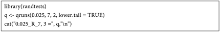RSUE facilitates the computation of these quantiles. To calculate them using the R program, the following script can be employed [3] , where the first number represents the order of the quantile, the second number is the parameter n₀, the third number is the parameter n₁, and “lower.tail = TRUE” is used for left-tailed calculations, while “lower.tail = FALSE” is used for right-tailed calculations.

5. Sampling Distribution and Decision with Large-Samples

The distribution of the number of runs tends to converge to the normal distribution [2] . When both n₀ and n₁ exceed 20 and n is greater than or equal to 30, preferably when both n₀ and n₁ exceed 20 and n is greater than 40, the asymptotic probability via the standard normal distribution can be employed [13] . This approximation becomes more accurate when the values of n₀ or n₁ are both close to and large [14] .

Initially, the mathematical expectation or arithmetic mean of the number of runs is computed from the normal distribution approximation [1] [2] using the formula in Equation (8). Subsequently, the standard deviation of the number of runs from the normal distribution approximation is determined [1] [2] using the formula in Equation (20).

$DE\left(R\right)=\sqrt{\frac{2\times n_0\times n_1\times \left(2\times n_0\times n_1-n\right)}{n^2\times \left(n-1\right)}}=\sqrt{\frac{\left(E\left(R\right)-1\right)\times \left(E\left(R\right)-2\right)}{n-1}}$ (20)

Following that, the test statistic Z, corresponding to the standardized number of runs, is derived [1] [2] using the formula in Equation (21).

$Z=\frac{r-E\left(R\right)}{DE\left(R\right)}=\frac{r-\left(\frac{2\times n_0\times n_1}{n}+1\right)}{\sqrt{\frac{2\times n_0\times n_1\times \left(2\times n_0\times n_1-n\right)}{n^2\times \left(n-1\right)}}}$ (21)

The Yates continuity correction can be applied by approximating a discrete distribution (number of runs) to a continuous (normal) distribution. This process is automated in the SPSS program [5] through the use of the formula in Equation (22).

$Z=\frac{\left(r\mp 0.5\right)-E\left(R\right)}{DE\left(R\right)}$ (22)

If |r − E(R)| ≤ 0.5 or n ≥ 50, the continuity correction (∓0.5) is omitted. For n < 50, the continuity correction is applied using the following algorithm: if r − E(R) < −0.5, 0.5 is added, and if r − E(R) > 0.5, 0.5 is subtracted.

The RSUE program offers an optional continuity correction, while the R program lacks an option for its implementation. It’s worth noting that the validity of the continuity correction, particularly the Yates continuity correction, has been a subject of debate [15] [16] [17] .

The test statistic Z follows a standard normal distribution: Z ~ N(0, 1). Decisions can rely on the critical values or quantiles of this distribution: if z_α/2 ≤ z ≤ z_{1− (α/2)}, H₀ holds; on the contrary, if z < z_α/2 or z > z_1−(α/2), H₀ is rejected.

In turn, the decision can be based on the probability value or critical level calculated using the standard normal distribution. When z ≤ 0, if 2 × P(Z ≤ z) ≥ α, H₀ holds and if 2 × P(Z ≤ z) < α, H₀ is rejected. When z > 0, if 2 × P(Z ≥ z) = 2 × [1 − P(Z < z)] ≥ α, H₀ holds and if 2 × [1 − P(Z ≤ z)] < α, H₀ is rejected.

6. Comparing Algorithms for Calculating the Two-Tailed Exact Probability

6.1. Method

Fifty-nine samples with dichotomous data were generated to compare the four algorithms, comprising 29 samples with an even number of data (n = 10) and 30 samples with an odd number of data (n = 11). See Table 5.

On the one hand, nine samples (r from 2 to 10) were derived from a distribution of the number of runs with parameters n₀ = n₁ = 5 (R5|5), eight samples (r from 2 to 9) from a distribution with parameters n₀ = 4 and n₁ = 6 (R4|6), six samples (r from 2 to 7) from a distribution with parameters n₀ = 3 and n₁ = 7 (R3|7), four samples (r from 2 to 5) from a distribution with parameters n₀ = 2 and n₁ = 8 (R2|9), and two samples (r from 2 to 3) from a distribution of parameters n₀ = 1 and n₁ = 9 (R1|9).

On the other hand, ten samples (r from 2 to 11) are drawn from a distribution with parameters n₀ = 5 and n₁ = 6 (R5|6), eight samples (r from 2 to 9) from a distribution with parameters n₀ = 4 and n₁ = 7 (R4|7), six samples (r from 2 to 7) from a distribution with parameters n₀ = 3 and n₁ = 8 (R3|8), four samples (r from 2 to 5) from a distribution with parameters n₀ = 2 and n₁ = 9 (R2|9), and two samples (r from 2 to 3) from a distribution with parameters n₀ = 1 and n₁ = 10 (R1|10).

The central tendency comparison of the two-tailed exact probabilities among the four algorithms, whose distributions deviated from normality, was conducted using Friedman’s test with a significance level of 5%. Post-hoc comparisons were performed using Conover’s test [13] with Benjamini-Yekutielli correction for the familywise error rate [18] . The effect size of the algorithm’s impact on the probabilities was estimated by Kendall’s W coefficient of concordance and the average Spearman’s rank correlation [13] .

Table 6 summarizes the computational processes of the four algorithms. It shows the criteria for defining the symmetry axis, how the two sides of the distribution are determined, as well as how the one-tailed and two-tailed probabilities are obtained.

6.2. Results: Calculation and Comparison of Probabilities

Table 7 shows the definition of the (left and right) sides of the 10 distributions of the number of runs. It includes one-tailed and two-tailed probabilities calculated using RSUE and R programs, along with mathematical expectations, exact point, and cumulative probabilities for these distributions. The R program uses mathematical expectations for defining distribution sides, while the RSUE program relies on the median.

Table 8 presents the calculations for one-tailed and two-tailed probabilities using the SPSS programs and the new proposal.

The analysis revealed a significant difference among the four algorithms (Friedman Q-statistic = 58.890, df = 3, p-value < 0.001; Iman-Davenport

Table 5. Generated samples.

Note. Each sample is identified by the parameters n₀ and n₁ of the R distribution from which it is drawn and its number of runs (r). Runs test: n = n₀ + n₁ = sample size, n₀ = number of zeros, n₁ = number of ones, r = number of runs (threshold: 0.5).

Table 6. Synthesis of the calculation of the one- or two-tailed exact probability using the four algorithms.

Note. RSUE = Real Statistics using Excel, r = number of runs, varying from 2 to Max(R) = n₀ + n₁ when n₀ = n₁ or 2 × min(n₀, n₁) + 1 when n₀ ≠ n₁, E(R) = mathematical expectation and Mdn(R) = median of the number of runs distribution with parameters n₀ and n₁. * If there is no equal or greater probability, the one-tailed probability is doubled to obtain two-tailed probability, unless there is extreme negative skewness (A_B = −1). In this case, the probabilities corresponding to the other tail of the values of R in the lengthened tail are 0 and, with the value of R in the shortened tail, the one-tailed probability is doubled with the restriction that the maximum value of the two-tailed probability is 1.

Table 7. One-tailed and two-tailed exact probability with RSUE and R programs.

Note. Each sample is identified by the parameters n₀ and n₁ of the R distribution from which it is drawn and its number of runs (r), n = n₀ + n₁ = sample size, n₀ = number of zeros, n₁ = number of ones, r = number of runs (threshold: 0.5).

Table 8. One-tailed and two-tailed exact probability with RSUE and R programs.

Note. Sample: n₀|n₁_r = parameters: n₀ (numbers of 0 s) and n₁ (numbers of 1 s), and r = number of runs, p = probability value. |r − E(R|n₀, n₁)| = absolute difference of the number of runs r and the mathematical expectation of the distribution of the number of runs; a horizontal line separates the two sides of the distribution. Mdn (R R|n₀, n₁) = median of the distribution of the number of runs. Sk_B = Bickel’s skewness coefficient based on the mode.

Table 9. Differences between the two-tailed exact probabilities of the four procedures.

Note. E = Real Statistics using Excel, R = R program, SPSS = Statistical Package for the Social Sciences, N = new proposal. Frequency: <0 (number of negative differences), = 0 (number of null differences or equivalences), and >0 (number of positive differences). Pairwise comparisons using Friedman-Conover test with Benjamini-Yekutielli correction for familywise error: MD = mean signed differences of two-tailed exact probabilities, DRM = difference in mean ranks, SE = standard error of difference in mean ranks, t-statistic = DRM/SE = DRM/0.188, p-value = two-tailed probability value following a t-distribution with 174 degree of freedom, α_c = corrected significance level, significance: “yes” when p-value is less than α_c and “no” when p-value is greater o equal than α_c.

F-statistic = 28.919, df₁ = 3, df₂ = 174, p-value < 0.001). The effect size was medium (Kendall’s w = 0.333, ${\bar{r}}_S$ = 0.321). Utilizing Conover’s test with the Benjamini-Yekutieli correction, significant differences of central tendency in probability were observed between RSUE and the R program (RSUE < R), as well as the new proposal (RSUE < NP), and similarly between SPSS and the R program (SPSS < R) and the new proposal (SPSS < NP). The central tendencies in probability between RSUE and SPSS, as well as between R program and the new proposal, were found to be statistically equivalent (Table 9).

7. Conclusions

It is important to acknowledge that the computation employed by RSUE assumes symmetry, a condition valid only when n₁ = n₂. Moreover, RSUE treats the distribution of the number of runs as an analog of the normal distribution, which is continuous and symmetrical, when this distribution is discrete and exceptionally symmetrical. Accordingly, RSUE uses the median as axis of symmetry instead of the mathematical expectation. This analogy may be based on the distributional convergence to the normal distribution [2] . However, with small samples, the approximation is not appropriate [14] . When employing this algorithm, it emerges that both the one-tailed and two-tailed probabilities of the maximum value of R are zero. This implies that the lowest mean results when averaging the exact two-tailed probabilities of the 59 samples. It should be noted that the fact that the one-tailed and two-tailed probability is always zero at the maximum r value when the point probability is not zero is a contradiction, and constitutes a further inconsistency with this program.

The SPSS program’s algorithm employs the mathematical expectation as the axis of symmetry to delineate the two sides of the distribution and determine the value of r corresponding to the opposite side. The sum of the one-tailed probabilities of r and its counterpart on the other side yields the two-tailed probability. The proposed algorithm shares similarities but defines the distribution’s two sides using the median. It employs quantile order on the left side and the complementary quantile order on the right to ascertain the probability corresponding to the opposite tail, except for the median, where its complement represents the probability of the other tail. The summation of both probabilities provides the exact two-tailed probability, which is more accurate given the varied asymmetry situations presented by the distribution of the number of runs, including extreme negative asymmetry [9] . However, both procedures are more suitable than doubling the one-sided probability, as performed by the R program. Doubling the one-sided probability fails to adequately consider the asymmetry characteristics of the distribution of the number of runs and may result in probability values exceeding 1.

In the central tendency comparisons, the proposed algorithm is slightly more conservative with the null hypothesis of randomness than the SPSS program. It is a general characteristic of robust procedures [19] , although it may be perceived as a drawback in terms of decisions relying on exact probability [20] [21] [22] .

This study generated various samples, utilizing a predefined cut-off point to ensure that the sum of n₀ and n₁ consistently equaled the sample size (n) across different programs. The goal was to simulate the behavior of the distribution of the number of runs. Thus, when n₀ = n₁, the exact two-tailed probabilities of the four procedures coincide, except in the case of the RSUE when r = n = 10.

However, even when n₀ = n₁, there are discrepancies in the exact two-tailed probabilities between RSUE, SPSS, and R program. This discrepancy arises because R program and RSUE exclude sample values equal to the cut-off point, whereas SPSS does not. The exclusion of values equal to the cut-off point is justified as a correction for ties, a common practice when assigning ranks [23] . This correction aims to enhance the power of non-parametric tests, akin to the continuity correction. However, its effectiveness remains debatable [24] , leading to varied implementation across programs, with some adopting it and others abstaining [4] .

An option not explored in this study is the calculation of probability through bootstrapping. The SPSS program includes this functionality, albeit limited to the Z statistic of the asymptotic approximation, which is suitable for large samples. For small samples, the true choice is exact probability [3] [6] , as bootstrap is not recommended for small samples [25] . This underscores the significance of the present study.

As limitations of the study, it should be noted that only three programs have been considered, though others like C#, BMDP, SAS, STATISTX, GNU/Octave also include the runs test. Moreover, two sample sizes were chosen: even (10 data points) and odd (11 data points). This simplification is assumed to be adequate, representative, and clear for comparing exact two-tailed probabilities computed by the four algorithms.

In conclusion, the calculation provided by SPSS and the new proposal is deemed more suitable when compared to the calculations of the RSUE and R programs. The new proposal represents a robust and well-supported calculation procedure, albeit slightly more conservative than the SPSS method. Additionally, it has the potential for generalization to other tests, including binomial and sign tests.

Acknowledgements

The author thanks the reviewers and editor for their helpful comments.

Conflicts of Interest

The authors declare no conflicts of interest regarding the publication of this paper.

References

[1]	Wald, A. and Wolfowitz, J. (1943) An Exact Test for Randomness in the Non-Parametric Case Based on Serial Correlation. The Annals of Mathematical Statistics, 14, 378-388. https://doi.org/10.1214/aoms/1177731358
[2]	Wald, A. and Wolfowitz, J. (1940) On a Test Whether Two Samples Are from the Same Population. The Annals of Mathematical Statistics, 11, 147-162. https://doi.org/10.1214/aoms/1177731909
[3]	Caeiro, F. (2022) Package “Randtests”. https://cran.r-project.org/web/packages/randtests/randtests.pdf
[4]	Zaiontz, C. (2016) One-Sample Runs Test. Real Statistics Using Excel. https://real-statistics.com/non-parametric-tests/one-sample-runs-test/
[5]	IBM Corporation (2013) IBM SPSS Statistics 22 Algorithms. https://www.sussex.ac.uk/its/pdfs/SPSS_Statistics_Algorithms_22.pdf
[6]	IBM Corporation (2022) SPSS Statistics 29. Documentation. https://www.ibm.com/docs/en/spss-statistics/29.0.0
[7]	Mehta, C.R. and Patel, N.R. (2013) IBM SPSS Exact Tests. https://www.ibm.com/docs/en/SSLVMB_27.0.0/pdf/en/IBM_SPSS_Exact_Tests.pdf
[8]	Mohajan, H.K. (2020) Quantitative Research: A Successful Investigation in Natural and Social Sciences. Journal of Economic Development, Environment and People, 9, 50-79.
[9]	Gunver, M.G., Senocak, M.S. and Vehid S. (2018) To Determine Skewness, Mean and Deviation with a New Approach on Continuous Data. Ponte: International Scientific Researches Journal, 73, 64-79. https://doi.org/10.21506/j.ponte.2018.2.5
[10]	Verma, J.P. and Abdel-Salam, A.-S.G. (2019) Testing Statistical Assumptions in Research. John Wiley and Sons, Hoboken.
[11]	Poncet, P. (2022) Package Modeest. Mode Estimation. https://cran.r-project.org/web/packages/modeest/modeest.pdf
[12]	Bickel, D.R. (2002) Robust Estimators of the Mode and Skewness of Continuous Data. Computational Statistics & Data Analysis, 39, 153-163. https://doi.org/10.1016/S0167-9473(01)00057-3
[13]	Conover, W.J. (1999) Practical Nonparametric Statistics. 3th Edition, John Wiley and Sons, Hoboken.
[14]	Diamantopoulos, A., Schlegelmilch, B. and Halkias, G. (2023) Simple Things First: One Variable, One Sample. In: Taking the Fear out of Data Analysis, Edward Elgar Publishing, Cheltenham, 163-184. https://doi.org/10.4337/9781803929842.00022
[15]	Alvo, M. (2022) Nonparametric Statistics. In: Statistical Inference and Machine Learning for Big Data, Springer International Publishing, Cham, 95-170.
[16]	Kvam, P., Vidakovic, B. and Ki, S.-J. (2022) Nonparametric Statistics with Applications to Science and Engineering with R. John Wiley and Sons, Hoboken.
[17]	Martín Andrés, A., álvarez Hernández, M. and Gayá Moreno, F. (2023) The Yates, Conover, and Mantel Statistics in 2 × 2 Tables Revisited (and Extended). Statistica Neerlandica. https://doi.org/10.1111/stan.12320
[18]	Benjamini, Y. and Yekutieli, D. (2001) The Control of False Discovery Rate in Multiple Testing under Dependency. Annals of Statistics, 29, 1165-1188. https://doi.org/10.1214/aos/1013699998
[19]	Maronna, R.A., Martin, R.D., Yohai, V.J. and Salibián-Barrera, M. (2019) Robust Statistics: Theory and Methods (with R). 2nd Edition, John Wiley & Sons, Hoboken.
[20]	Bind, M.A. and Rubin, D.B. (2020) When Possible, Report a Fisher-Exact p Value and Display Its Underlying Null Randomization Distribution. Proceedings of the National Academy of Sciences, 117, 19151-19158. https://doi.org/10.1073/pnas.1915454117
[21]	DiCiccio, C.J., DiCiccio, T.J. and Romano, J.P. (2020) Exact Tests via Multiple Data Splitting. Statistics & Probability Letters, 166, Article ID: 108865. https://doi.org/10.1016/j.spl.2020.108865
[22]	Frey, J. and Zhang, Y. (2019) Improved Exact Confidence Intervals for a Proportion Using Ranked-Set Sampling. Journal of the Korean Statistical Society, 48, 493-501. https://doi.org/10.1016/j.jkss.2019.05.003
[23]	Hodges, C.B., Stone, B.M., Johnson, P.K., Carter III, J.H, Sawyers, C.K., Roby, P.R. and Lindsey, H.M. (2023) Researcher Degrees of Freedom in Statistical Software Contribute to Unreliable Results: A Comparison of Nonparametric Analyses Conducted in SPSS, SAS, Stata, and R. Behavior Research Methods, 55, 2813-2837. https://doi.org/10.3758/s13428-022-01932-2
[24]	McGee, M. (2018) Case for Omitting Tied Observations in the Two-Sample T-Test and the Wilcoxon-Mann-Whitney Test. PLOS ONE, 13, e0200837. https://doi.org/10.1371/journal.pone.0200837
[25]	Rousselet, G., Pernet, C.R. and Wilcox, R.R. (2023) An Introduction to the Bootstrap: A Versatile Method to Make Inferences by Using Data-Driven Simulations. Meta-Psychology, 7, Article No. 2058. https://doi.org/10.15626/MP.2019.2058