Calabi-Yau Topology of Primordial Fermions

Edwin Eugene Klingman

Cybernetic Micro Systems, Inc., San Gregorio, CA, USA.

DOI: 10.4236/jmp.2024.151005                

Abstract

Quantum field theory creates fermions via abstract operators exciting abstract fields, with a specific field for each type of specific particle. This operator algebra lends itself well to quantum statistics, nevertheless, our physical understanding of this process is nonintuitive at best. In this paper we analyze the creation of fermions from primordial gauge field quantum gravity loops in the context of Calabi-Yau manifold theory. I extend a prior mass-gap treatment based on Yang-Mills gauge theory of higher order self-interaction to include the half-integral spin of fermions.

Keywords

Calabi-Yau Topology, Fermion Spin, Particle Genesis, Primordial Field, Self-Interaction Equations, Yang-Mills Gravity

1. Introduction

Fermions, generally identified as the matter in our Universe, are characterized by a finite mass-gap above the vacuum and by ½ -integer spin. There is currently no understanding of the creation of matter, meaning fermions with mass, spin, and charge. The Millennium $1,000,000 Mass gap Prize asks for an explanation of why particle masses don’t decay to vacuum energy. The lowest stable particle energy over the vacuum is the mass gap in question. The Standard Model of Particle Physics does not know how to compute particle masses; they are put in by hand. Mass is tricky in quantum field theory, which is based on the concept of a specific field distributed throughout space for each type of particle. Stimulating the field is considered to bring the particle into existence. How mass evolved is a mystery. Quantum fields cannot be measured, and their physical nature is unknown; both epistemic and ontological interpretations exist.

Sbitnev [1] , using quaternions for translation in 4D space and spin rotation on 3D spheres, deals with a space densely filled by an incompressible quantum superfluid; a Bose-Einstein condensate. Computations on this fluid lead to gravitomagnetic equations similar to Maxwell’s equations for electromagnetic fields: “Schrödinger, vorticity, and wave equations follow from these equations as a natural outcome.” Sbitnev’s approach differs from primordial theory based primarily on ontological assumptions. For example, $\rho \left(r,t\right)$ is the density distribution of “sub-quantum particles, carriers of masses”; no such sub-quantum particles exist in primordial theory. Also, “Physical vacuum is a special super fluid medium populated by enormous amounts of virtual particle-antiparticle pairs”, while virtual pairs do not exist in primordial theory. Further, Sbitnev introduces a torus with a string twisting two times around the torus tube, then maps this (in a physically impossible way) into a 3D sphere and draws conclusions about spin. “The frequency ω is that of rotation about the center of the torus; the toroidal vortex wall can be filled by helicoidal strings.” Strings do not exist in primordial theory. Rather than zero viscosity, Sbitnev considers dynamical “viscosity that fluctuates about zero in time. …we believe that it is zero in the average in time, but its variance is not zero.” He further believes that this viscosity $\mu$ avoids a singularity at the vortex core and supports infinite lifetime of the vortex. Based on $\Omega =c{\rho }_m\omega$ , he observes that the vorticity equation ${\rho }_m\frac{\partial \omega }{\partial t}=\mu \left(t\right){\nabla }^2\omega$ describes vortex motion in a local reference frame sliding along an optimal trajectory guided by the wave function that is solution of Schrödinger’s equation, ideally simulating the particle moving along the Bohm trajectory. In summary, Sbitnev treats gravito magnetism with quantum fields per particle and with vacuum as virtual particle-antiparticle pairs. Finally, Sbitnev assumes the “weak field approximation”, a crucial mistake made by physicists for over a century.

Quantum field theory is well defined, so it is relatively easy to compare to primordial field theory, which is explicitly based on an ontological model of the physically real primordial field (that all modern theories assume that all forces converge to.) Quantum interactions occur between fields/particles and the system evolves through these interactions; primordial field evolution is possible only through self-interaction; nothing else exists to interact with. Quite simply, the change in state of the system, represented by $\nabla$ acting on the system, is equal to the system acting on itself, hence:

$\nabla \psi =\psi \psi \Rightarrow \psi \left(\xi \right)=-{\xi }^{-1},\psi \left(\xi \right)={\xi }^{-1}$ (1)

with ${\nabla }_{\xi }={\partial }_{\xi }$ . Solutions to the self-interacting equations include inverse scalar and inverse vector; interpreted as time and space, these yield duration and distance, both applicable to fields. Primordial theory considers only one field to exist, with aspects based on space $\psi \left(\xi \right)=\frac{1}{r}$ and time $\psi \left(\xi \right)=-\frac{1}{t}$ , and dynamics based on turbulence of the ultra-dense field. Via Hestenes’ Geometric Calculus operating on $\psi =G+iC$ we derive Heaviside’s gravitomagnetic dual of Maxwell’s electromagnetics. The important self-interactions are those of a given momentum density interacting with field circulations induced by the momentum density, formulated on a fractional lattice [2] .

Primordial field theory has no undefined entities such as the quantum fields and wave functions of quantum field theory; there is only the reality of the gravitomagnetic field. Sbitnev neglects charge in his treatment of spin; we will derive electromagnetic charge in primordial field theory. First, we examine the issue of fermion spin.

In primordial field theory the primordial field is the real physical gravitomagnetic force field that interacts with moving mass density. In the beginning the density of mass-energy was essentially as high as we wish it to be. Since particle creation occurs at LHC energy densities, we already know the relevant range of energies; consider the collision-event-resulting-jets simply to be a case of the primordial field in action, induced via mind boggling instrumentation. In 2006, as I began primordial field theory, the LHC was in process of reassessing their expected “quark gas” in the collisions to be instead a perfect fluid. This very real particle phenomena is derived in primordial field theory through the self-interaction process. Self-linking turbulence involves varying energy distribution, and momentum density induces circulation in the local C-field. The key equation is $\nabla \times C=-\rho v+\frac{\partial G}{\partial t}$ with $g=c=\hslash =1$ . The field energy density $\rho$ moving through local gravity $G$ (the ether) induces circulation $\nabla \times C$ . This circulation induces a higher order circulation, as the field interacts with itself. My quantum loop gravity fractional lattice treatment of this interlinked torus system has been shown to produce a stability zone in which collapse to a primal torus is energetically favored. I formulate this as a mass gap “existence proof”, analyzing mass-gap in terms of higher-order self-interactions of the primordial field by reinterpreting the non-Abelian term of Yang-Mills gauge theory as follows: $\left[A_{\mu },A_{\nu }\right]\Rightarrow \left[A_{\mu }^{\left(i\right)},A_{\mu }^{\left(i+2\right)}\right]$ adapting it to higher-order self-interaction. In this paper we assume this mass-gap existence proof establishes the fundamental requirement and we analyze the fermion spin in the context of Calabi-Yau theory.

A quantum theorist may wonder, “why introduce Calabi-Yau?” The answer is subtle, but for the most part it means that I do not have to prove my statements. Calabi-Yau provides a framework of proof and defines the limits and constraints of the framework: as long as I remain in the framework, my statements are true. For example, Sbitnev introduces a torus with a “string”, which he claims twists two times around the torus tube, then he proceeds to map this into a physically impossible 3D sphere. But as there is ever-more reason to doubt the efficacy of string theory, I prefer to have a specific mathematico-logical framework in mind and Calabi-Yau theory provides exactly that framework. The decision to remain within the bounds of a compact Kahler manifold, with a vanishing first Chern class, allows one to assume a Ricci-flat metric. Hestenes’ Geometric Calculus applies on a Ricci-flat metric, as well as Wolfram’s Mathematica-based 3D perspectives.

In short, Primordial field theory differs significantly from Quantum field theory, which assigns an individual quantum field existing at every point in space-time for each class of elementary particle. Specific particles are invoked via particle creation operator and viewed as excitations in a specific field; when Feynman developed his quantum field theory of gravity, he began by assuming “gravity as the 31^st field” [3] . Creation of such particles is nonintuitive; operator algebra enables physics in which the total number of particles changes based on harmonic oscillators and provides an abstract means of creating and annihilating specific particles, based on specific fields. Elsewhere I develop an intuitive understanding of particle creation from the primordial field of the universe, involving new concepts of physics. Many physicists, comfortable with complex, albeit nonintuitive, theories, tend to dismiss intuitive approaches to any complex problem they are familiar with, so I formulate the theory in terms of Einstein’s field equations, Yang-Mills gauge theory, and now Calabi-Yau topology, these being familiar approaches that have failed to deliver the goods but are felt to be generally valid approaches to the problem. The structure of this Letter is as follows:

Sec. 2 The ontology of time and space is introduced. We ask if there could be gravity in a universe devoid of matter (no particles)?

Sec. 3 The theory of the primordial field of our Universe, prior to the creation of matter.

Sec. 4 The Calabi conjecture is framed in terms of a metric, the geometry of a space, and such a metric, derived in 1921 by Kasner, yields an exact solution to Einstein’s field equations, interpreted herein in terms of the dynamical primordial field.

Sec. 5 Review of primordial field equation in the Kasner metric and higher order self-interaction physics. Re-interpreting the Yang-Mills nonabelian terms yields a mass-gap existence proof.

Sec. 6 Topological aspects of the Calabi-Yau manifold, including Kahler geometry, first class Chern, complex manifolds, and Ricci curvature.

Sec. 7 Primordial flow analyzed in Calabi terms.

Sec. 8 Ontological flow on a torus.

Sec. 9 Separation of U(1) × U(1) flow symmetry.

Sec. 10 Derivation of Quantum Spin.

Sec. 11 Parallel vector transport around a closed path shows ½ -integral character of this flow.

Sec. 12 Measurements on a dynamic model.

Sec. 13 Summary.

Sec. 14 Conclusions.

2. The Ontology of Time and Space

Laurent Field states [4] : “Spacetime is just an abstraction…. I believed all my life that spacetime exists, but I no longer do so.” Einstein early concluded that space and time are abstractions; “there is no vacuum [aka ‘empty space’] absent field.” [5] . He later concluded that the field is effectively the ether through which waves propagate but did not, however, go back and fix special relativity; he instead introduced curved space, which dominated physics for a century. In curved space local gravitational energy density is undefined; instead, we have variations of “quasi-local-mass”. I treat these conflicting concepts in terms of Heaviside’s gravitational equations derived from the primordial field self-interaction principle [6] .

Relevant to these concepts is Ricci curvature, which corresponds to a space with no matter. Calabi, a geometer, asked if there could be gravity in our universe even if space is a vacuum totally devoid of matter [7] . If so, he saw that curvature makes gravity without matter possible. In the following we review the geometer’s approach to this (essentially physics) problem and attempt to clarify problematic areas of this conjecture: we identify “matter” with “particles”, specifically fermions, while we identify “the vacuum” as the primordial field.

3. The Primordial Field of the Universe

The standard model of particle physics assumes all forces merge into one at the big bang, though this has not been demonstrated. Our fundamental assumption is that the primordial field, and nothing but the primordial field, existed at the Creation. If interaction is to occur (as it must, to evolve to our current Universe) the field must interact with itself; nothing else exists to interact with. This Self-Interaction Principle is represented by the Self-Interaction equation $\nabla \psi =\psi \psi$ where $\psi$ represents the primordial field and $\nabla$ represents the change operator. If the field depends upon some parameter $\xi$ , the change operator becomes $\nabla \to {\partial }_{\xi }$ , which leads to two formal solutions: a scalar solution $\psi \left(\xi \right)=-{\xi }^{-1}$ and a vector solution $\psi \left(\xi \right)={\xi }^{-1}$ , associated respectively with time t and position $r$ . Defining primordial field $\psi =G\left(r,t\right)+iC\left(r,t\right)$ with corresponding operator $\nabla =\nabla +{\partial }_t$ , Equation (1) becomes

$\left(\nabla +{\partial }_t\right)\left(G+iC\right)=\left(G+iC\right)\left(G+iC\right)$ (2)

A Hestenes’ Geometric Calculus expansion of this equation immediately leads to the following:

Self-Interaction equations Heaviside equations

$\nabla \cdot G=G\cdot G-C\cdot C$ $\nabla \cdot G=-\rho$

$i\nabla \cdot C=i2G\cdot C$ $\nabla \cdot C=0$ (3)

${\partial }_{t}G-\nabla \times C=G\times C\pm C\times G$ $\nabla \times C=-\rho v+{\partial }_{t}G$

$i\nabla \times G+i{\partial }_{t}C=0$ $\nabla \times G=-{\partial }_{t}C$

The terms on the left are given field energy density interpretation leading to Heaviside’s 1893 formulation [8] of the right side of (3) with $\hslash =g=c=1$ . These equations are identical (under iteration) to Einstein’s non-linear field equations. Self-interaction Equations (3) derive from (2) in straightforward fashion. To obtain the right-hand side physical meaning is attached to field $\psi$ , with $G$ gravity and $C$ the gravitomagnetic field. The concept of field strength is absent in the derivation, other than the implicit assumption of strong fields existing at the big bang. When Heaviside’s equations are derived by linearizing Einstein’s equations (discarding higher order terms) the resultant equations are erroneously labeled the weak field approximation to Einstein’s equations, leading physicists to regard Einstein’s geometric equations as the “true” physics with Heaviside believed to hold only for weak fields. Since our Heaviside formulation is equivalent to Einstein at all field strengths; these equations of gravity hold at all scales, including the particle scale, geometry-based concepts of gravity are abstract and unnecessary for a theory of gravity; despite the common assumption that gravity depends on mass, Heaviside’s equations clearly show that the actual dependence is on mass density $\rho$ . The equations of gravity (3) are based on gravitational fields $G\left(r,t\right)$ and $C\left(r,t\right)$ while Yang-Mills is based on gauge fields. Field equation $\nabla \cdot C=0$ implies we can make use of vector identity $\nabla \cdot \nabla \times A=0$ to replace $C$ with vector $\nabla \times A$ . Compatible with Equations (3) are gauge field equations:

$C=\nabla \times A$ , $G=-\nabla \varphi -{\partial }_{t}A$ , ${\partial }_t\varphi +\nabla \cdot A=0$ (4)

The first two Equations in (4) define the fields in terms of the four-potential A, while the last eqn specifies the Lorenz gauge condition, ${\partial }_{\mu }{A}^{\mu }=0$ . The scalar potential $\varphi =-m/r$ , and vector potential $A=v$ ; gauge field $A$ is seen to be a velocity field $v$ . Expansion of the gauge field equation allows us to interpret the Abelian form of the field strength: $F_{\mu \nu }={\partial }_{\mu }{A}_{\nu }-{\partial }_{\nu }{A}_{\mu }$ . The field strength tensor constructed from the above is shown [9] :

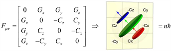(5)

Figure 1. The C-field momentum-energy density matrix.

Ten coefficients are needed to describe how metric coefficients change from point to point in the manifold. In Figure 1, the Heaviside field tensor is symmetrical about the 4 × 4 diagonal, with two sets of six numbers on either side of the diagonal. Gravitomagnetic terms $C_y=C_{xz}$ and $-C_y=C_{zx}$ represent bivectors rotating in the xz-plane equi­valent to the rotation about the axial vector on the y-axis. If $g=c=1$ the C-field is described by $C=r\times p$ where $p$ is the momentum density inducing circulation equivalent to angular momentum density ( $L=r\times p$ ). In the Einstein-deHaas sense, gravitomagnetic field $C$ essentially is angular momentum. At particle scale we expect this inherent spin density field to be quantized, as implied in Figure 1. Were this not the case, a C-field vortex, like a skater pulling in her arms to zero, would spin up to infinite density at a point. Thus, we anticipate an extended object, not the point particles of quantum field theory.

The formulation $F^{\mu \nu }={\partial }^{\mu }{A}^{\nu }-{\partial }^{\nu }{A}^{\mu }$ separates radial field $G\left(r\right)$ and gravitomagnetic field $C\left(r\right)$ , with gravitomagnetic terms representing angular momentum. Planck’s constant has dimensions of angular momentum $\hslash =m{l}^2/t=mvr$ , so this is a feasible underlying degree of freedom to be quantized. If gravity does not interact with itself in a static situation, one must ask what Yang-Mills non-Abelian term $\left[A_{\mu },A_{\nu }\right]$ represents. It has not been interpreted in any useful fashion dynamically, so our mass-gap existence proof attempts a new interpretation of self-interaction in Yang-Mills. This is justified by the fact that almost seventy years of work in this field has failed to solve the critical problems. This is perhaps hinted at with a quote from Taubes:

“Once upon a time a Martian arrived, gave us the Yang-Mills equations, and left.”

Jaffe and Witten define the mass gap problem [10] and note: “Some results are known for Yang-Mills theory on a 4-torus T ⁴ approximating R ⁴ and, while the construction is not complete, there is ample indication that known methods could be extended to construct Yang-Mills on T ⁴.” The existence proof approach for a solution to the mass-gap problem [11] will now be used to explore the issue of ½ integral spin.

4. The Calabi Conjecture

Yau observes that Einstein’s equations tie curvature to gravity. This century old concept has been accompanied by century old paradoxes, of the type associated with the concept of “quasi-local-mass” [12] . How physical energy density can be encoded as geometry is explained in [13] . Our goal here is to employ topology and geometry on the primordial field ontology.

Calabi’s conjecture is concerned with spaces that have a specific type of curvature known as Ricci curvature, relating to the distribution of matter within the space. A space is Ricci-flat if space holds no matter. Eugenio Calabi, a geometer, viewed the problem as “strictly geometry” and therefore framed the problem in terms of a metric, i.e., the geometry of a space, defining the length of every path, in terms of distance between points in space. However, a given topological space can have many possible shapes and many possible metrics, so Yau concludes that Calabi’s conjecture concerning what kind of metric a space can “support” is equivalent to asking, “For a given topology, what kind of geometry is possible?”

We are now dealing with ontological concepts of physics such as vacuum, field, matter, energy density, and abstract concepts of geometry such as metric, topology, curvature, and manifold. We begin with a specific physics problem, the universe defined by the Kasner metric, then analyze it in terms of topological concepts.

5. The Dynamic Universe Defined by the Re-Interpreted Kasner Theory

We assume that the primordial field was present at the moment of Creation and expanded as the big bang. Perhaps initially only spherical symmetry applied, $G$ , but at some point, this symmetry broke, and the field became ultra-turbulent, with vortices and tori representing C-field angular momentum density distributions. Physically real turbulent loops twist in 3D and intersect themselves; such reconnection events realign forces—both energy and momentum proceed in opposite directions along the reconnection axis. Such an event has been used to initiate analysis of the Kasner metric, an exact solution to the Einstein field equation. In [14] I construct the physics of $h_{ij}$ for a dynamic spatially homogenous anisotropic Bianchi vacuum model that solves Einstein’s equations in terms of the physically real primordial field, otherwise devoid of matter. Kasner derived the solution to $R^{\mu \nu }=0$ in 1921. Narlikar and Karmarkar’s later formulation is:

$\text{d}{s}^2=c^2\text{d}{t}^2-{\displaystyle \underset{j=1}{\overset{D-1}{\sum }}{\left(1+nt\right)}^{2p_j}\text{d}{x}_j^2}$ . (6)

While Equation (6) is subject to constraints on $p_j$ , the meaning of parameter n has been obscure. I interpret n to be primordial field $C\left(t\right)$ induced by momentum $p_j$ , assumed to exist because of a reconnection event. In Figure 2(a) $r\left(x,y,z\right)$ is the point in space where the induced C-field is measured, while Figure 2(b) displays a C-field energy-density histogram based on axial symmetry associated with an arbitrary slice through the energy density history at $r\left(t\right)$ . An arbitrary slice of the field shows self-induced field behavior, with first and second order induction diagrammed in Figure 2(c).

The higher-order self-interaction shown in Figure 2(c) is treated elsewhere, but the matter-free field has energy density distribution that is turbulently dynamic. This contrasts with the static metrics of the one-body theory of general relativity such as Schwarzschild and Kerr. The Schwarzschild metric is $\text{d}{s}^2=g_{\mu \nu }\text{d}{x}^{\mu }\text{d}{x}^{\nu }=\left(1+2\varphi \right)\text{d}{t}^2-\left(1-2\varphi \right)\left(\text{d}{x}^2+\text{d}{y}^2+\text{d}{z}^2\right)$ where $\varphi ~m/r$ is a function only of position. In other words, the static metric is not a function of time; distribution of the field is fixed in space over all time. The dynamic metric (Equation (6)) is best understood as dynamically describing the distribution of the field over time, when $n\ne 0$ , due to the effect of the momentum density $p$ of the field. When $n=0$ the Kasner metric reduces to Euclidean space since ${\left(1\right)}^{2p}=1$ is always unity. However, if we assume that momentum density $p$ is non-zero, then our interpretation of the n term as the value of the local C-field induced by $p$ implies that n cannot be zero.

Kasner is a spherical topology in the sense that the boundary of the field can be deformed to a sphere. The constraints on the Kasner metric include a geometry in which the distributed field lengthens in one direction while shrinking in the other two directions, and vice versa. Momentum constraints ${\displaystyle \underset{j=1}{\overset{D-1}{\sum }}{p}_j}=1$ and ${\displaystyle \underset{j=1}{\overset{D-1}{\sum }}{p}_j^2}=1$ determine the specific shape. Kasner topology of a primordial field universe is not sufficient for creation of a fermion; the mass-gap existence proof relies upon local ultra-high-density field turbulence (found at the big bang or in atom-atom collisions at LHC) to assume evolution of a vortex-to-helix-to-torus topology, hence we next investigate topological concepts applicable to Calabi-Yau.

(a) (b) (c)

Figure 2. (a) C-field energy is calculated at position $r$ with respect to a reconnection event in an anisometric open universe described by the Kasner metric. (b) An energy history of two such induced C-field circulations. The time axis is mapped onto the reconnection axis corresponding to the z-axis, and cylindrical symmetry is applied. (c) An arbitrary slice through the momentum axis reveals second and third order induced C-field flows.

6. The Topology of Calabi-Yau

A manifold is a space or surface of any dimension n; the number of two-dimensional spaces is restricted to two basis types: either a sphere or a donut. The dynamic Kasner solution developed above represents a universe composed of nothing but a primordial field. Unlike the Schwarzschild solution, the cosmological Kasner solution does not have an “outside”; the surface or boundary of this universe is such that all the primordial field is “inside” the boundary, deformable into a sphere. In the Kasner solution the field is such that the distribution of field energy expands or contracts anisotropically; as noted, two dimensions increase in length, while one decreases, or vice versa. Conversely, the mass-gap solution has donut topology, specifically a one-hole torus. The Kasner spherical topology of the primordial universe differs from the local toroidal topology of the fermion, so relevant topological concepts are examined. Per Yau:

“Calabi wanted to know if a certain kind of complex manifold—a space that was compact and ‘Kahler’—that satisfied specific topological conditions (vanishing first Chern class) could have a Ricci-flat metric.”

Kahler: Manifolds resemble Euclidean space on a local scale but can be very different on a global scale. Calabi’s conjecture pertains strictly to complex manifolds—surfaces that are expressed in terms of complex numbers, i.e., two-dimensional local surfaces. Riemann surfaces are complex and automatically qualify as Kahler; space looks Euclidean at a single point and stays close to Euclidean when one moves away from the point. Such spaces are even-dimensional as only complex manifolds can have Kahler geometry, which provides an indication of how close a space comes to being Euclidean based on criteria that are not strictly related to curvature. Whether a particular metric is Kahler is a function of how the metric changes as one moves from point to point. Kahler manifolds are a subclass of complex manifolds known as Hermitian manifolds, “on which you can put the origin of a complex coordinate system at any point, such that the metric will look like a standard Euclidean metric at that point.” Kahler manifolds have a rotational symmetry such that vectors $\left(a,b\right)=a+ib$ on the manifold are rotated 90˚ via multiplication by the imaginary unit, i, with the length of the vector preserved. This “internal” symmetry supports parallel transport, as we will see in a following section. This internal symmetry, which in many ways defines Kahler manifolds, is restricted to the space tangent to the manifolds.

Internal symmetry: The “internal symmetry” of Kahler geometry is unrelated to the internal symmetry discussed in our Yang-Mills-based existence proof of the mass-gap. That internal symmetry refers to “iso-spin symmetry” which Heisenberg invented to allow use of Pauli’s SU(2) spin matrix algebra. Abstract iso-spin space differs from physical spin space, hence the qualification “internal space”. In Calabi-Yau space theory, “internal space” is instead associated with the six “hidden dimensions” (of a ten-dimensional string-theory formulation), assumed on the order of 10⁻³⁰ cm, modelled after Kaluza-Klein’s treatment of the 5^th dimension in their attempt to unify gravity and electromagnetics.

For the primordial field we choose 4-D constructions, rather than the 10-D or 11-D of string theory, which has been a center of interest in Calabi-Yau theory. Some string theorists make strong claims: “All of the numbers we measure in nature—all of the things we consider fundamental, such as the mass of quarks and electrons—all of these derive from the geometry of Calabi-Yau.” In this context, Calabi proposed an internal symmetry related to supersymmetry. Operation of LHC for over a decade has failed to show the slightest sign of super­symmetry, and Yau points out that, “…without supersymmetry, string theory makes little sense.” Our use of Calabi-Yau has nothing to do with supersymmetry.

Chern class: The next topological concept is Chern class, developed to mathematically characterize the difference between two manifolds. We are interested only in the simplest aspects dealing with complex manifolds. Specifically, we are interested in places where the flow in a vector field shuts down. For example, a spherical topology such as the earth supports the flow of wind currents at every point on the globe except two: there is zero net flow at the North pole and the South pole. These dead spots are places where nothing flows at all. The donut topology, on the other hand has no dead spots; flows around the surface of a torus can flow forever. Maxwell marveled at Helmholtz’s proof that “in a perfect fluid such as a whirling ring, if once generated, would go on whirling forever.” Clearly, we wish for our fermion flows to last forever—a topology in which this is the case is called a “vanishing Chern class” or “first Chern class of zero”.

Ricci curvature: Ricci curvature is essential to understanding what the Calabi conjecture is all about. It is a kind of average of a more detailed type of curvature known as sectional curvature. To find the Ricci curvature, pick a point on the manifold, find a vector tangent to that point, then look at all 2D tangent planes that contain that vector, each of which has a sectional (Gauss) curvature associated with the plane. The Ricci curvature is the average of these sectional curvatures. “A Ricci-flat manifold means that for each vector one picks, the average sectional curvatures of all the tangent planes containing that vector equals zero.” This, although the sectional curvature of any individual plane may not be zero. In higher dimensions a manifold can be Ricci-flat without being flat overall. Einstein’s formulation equates the flow of matter density and momenta at a point to the Ricci tensor. This is its key relevance for our theory of fermions so with these topological concepts in hand, we state the Calabi conjecture: “A compact Kahler manifold with a vanishing first Chern class will admit a metric that is Ricci-flat.”

Before using these geometer’s concepts to formulate a theory of spin, we review the physics of the same problem.

7. Analysis of Primordial Field in Calabi Terms

Having just reviewed the relevant Calabi-Yau topological concepts, we now relate these to the physics of the Ricci tensor. Einstein’s field theory equation

$R^{\mu \nu }=T^{\mu \nu }$ (7)

is unique in that the stress-energy tensor $T^{\mu \nu }$ is expressed in Euclidean space, whereas the Ricci tensor $R^{\mu \nu }$ represents curved space coordinates. Despite its endurance for over a century, this formulation makes no sense. No one knows how to solve an equation in which each side is formulated in a different coordinate system, one of which is unknown. One might ask, why not just express $T^{\mu \nu }$ in curved space? The problem is that the curvature is not known until after the problem has been solved. Feynman hints at this:

“In general, it is not possible to write down any kind of consistent $T^{\mu \nu }$ (…) unless one has already solved the complete, tangled problem.” (…) “Even for very simple problems, we have no idea how to go about writing down a proper $T^{\mu \nu }$ .”

Note that there is only one point common to both $T^{\mu \nu }$ and $R^{\mu \nu }$ —the point at the origin: (0, 0, 0). If we place a mass at this common point, the equation makes sense, and we can derive a solution, the Schwarzschild metric, based on the singularity at the origin. The field equation cannot be solved at the singularity, but does apply outside of the singularity, where $T^{\mu \nu }=0$ . Vishwakarma [15] , concluding that curvature of $R^{\mu \nu }$ is derived from the gravitation field outside the mass point, proposed that $T^{\mu \nu }$ is superfluous, and can simply be deleted from Einstein’s equation, leaving

$R^{\mu \nu }=0$ . (8)

That is, the stress-energy tensor representing energy density distributed over space, $T^{\mu \nu }$ , is nonsensical and has never been solved for or tested against general relativity experiments. In agreement with Vishwakarma’s conclusion that $R^{\mu \nu }$ curvature is based on the gravitational field, I have shown how the gravitational field energy density can be encoded as geometry (i.e., curvature), however, a proper energy-stress tensor of the gravitational field does not exist. This century-old paradox has led to such erroneous concepts as “quasi-local-mass”.

We consider next the left-hand-side of the field equation; starting with a Riemannian tensor, $R_{abcd}$ , we can obtain Ricci tensor $R^{\mu \nu }$ from the contraction $R_{ac}=g^{bd}{R}_{abcd}$ , where the sum over repeated indices is a bit like taking a scalar product of two vectors. In this case the shape of spacetime is defined by the metric tensor $g_{ab}$ with inverse such that $g^{ab}{g}_{ab}=\left[1\right]$ . The Ricci scalar is given by $R=R_{ac}{g}^{ac}$ . These are quantified expressions of spacetime curvature.

Consider a spherical region of closely spaced points around point P, moving with velocity $v$ . As the points flow through curved space the sphere can rotate, twist, or distort. The Ricci tensor $R_{ab}$ keeps track of the change in volume of the region. An associated Weyl tensor keeps track of the changes in shape of the region of points.

The fields of topology and physics converged when Yau realized that the Calabi-Yau conjecture need not be presented in purely geometric terms but can be written as a partial differential equation, whereas I start with differential equations and derive geometry (encoding energy density as geometry.) The differential equation he tried to solve in the Calabi-Yau conjecture is literally Einstein’s equation of empty space, ( $T^{\mu \nu }=0$ ), that is, Calabi-Yau manifolds are regarded as solutions to Einstein’s field equations.

Summarizing: Yau proved that a Ricci-flat metric can be found for compact Kahler space with a vanishing first Chern class; he could not produce a precise formulation of the metric itself. One is thus left, not with a solution, but merely an existence proof that a solution exists.

The simplest possible Calabi-Yau space is a two-dimensional torus or donut, compatible with the existence proof of the mass-gap, a torus derived from the use of Heaviside equations in turbulent media. Here we close with a simple topological “derivation” of the torus. (Figure 3)

Calabi’s conjecture is formulated in terms of complex manifold, Kahler geometry, metric, Chern class, Ricci curvature. Yau claims spaces satisfying the complicated set of topological demands are like rare diamonds, but the conjecture offers a general rule telling us that they are there.

(a) (b) (c)

Figure 3. A toric surface can be entire “flat” (zero Gauss curvature) because it can be made, in principle, by rolling up a sheet of paper into a tube and then joining the ends of the tube to each other.

8. Ontological Flow on a Torus

The above treatment has provided topological context and introduced existence proofs. I now analyze fermion topology in a 4D Calabi-Yau, modified Yang-Mills context, by focusing on the relevant ontological flow. Ignoring tangent bundles of differential geometry, we focus on the fact that the tangent space on the manifold can be defined as the set of all velocity vectors.

The solution to Maxwell’s field wave equations has U(1) symmetry, ${\text{e}}^{i\theta }~\cos \left(\theta \right)+i\sin \left(\theta \right)$ . In other words, the propagating field has helical structure. The physical regimes of interest are ultra-high-density gravitational fields, exemplified by big bang and atom-atom collisions at CERN. Both such regimes are extremely turbulent such that collisions of helices, including self-intersection occurs, potentially forming tori. In such cases the symmetry is U(1) × U(1).

Our mass-gap existence proof analyzes the self-interaction of a newly formed torus, concluding that beyond a certain stage of relaxation, the torus is self-stabilizing and self-healing against external interference and disturbances up to a limit. A key point on which we will construct our analysis is that Kahler manifolds are a subset of complex manifolds known as Hermitian manifolds, “on which you can put the origin of the complex coordinate system at any point, such that the metric will look like a standard Euclidean metric ${\eta }_{\mu \nu }$ at that point.” By implication, we could do so at any neighboring point, as well.

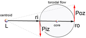
Consider the torus that is formed by “joining” the ends of a helical flow structure; the U(1) × U(1) structure is like circles surrounding every point on the torus “core” which is itself a circle. The surface of the donut represents the flow of the gravitomagnetic field energy density, described by the velocity vector, regarded as a vector being transported around a closed path. Topologically, this vector has the same direction as the tangent to the path at a given point. The tangent at any point on one of the U(1) circles is given as follows: For a curve with radius $r\left(t\right)$ the unit tangent vector $\hat{T}\left(t\right)$ is defined by $\hat{T}\left(t\right)=\stackrel{\dot{}}{r}/\left|\stackrel{\dot{}}{r}\right|$ . If we relabel this as $\stackrel{\dot{}}{r}/\stackrel{\dot{}}{s}$ where s is the arc length, then the tangent vector is given by $\frac{\text{d}r}{\text{d}s}$ , the change in the vector $r\left(t\right)$ as it moves along arc length.

Our U(1) × U(1) conceptual model shows every circle disconnected from every other circle; not a helix, (Figure 4). To reflect the physical ontology of the torus, we desire helical flow lines. The tangent, and hence flow velocity, has the same definition, and since the radius is constant around the U(1) circle, the velocity is constant. The parametric helix is $r=\left|r\right|\left\{\cos \left(t\right),\sin \left(t\right),t\right\}$ . This is easy to see, but for comparison with the torus we display it in Figure 5(b), according to the following:

x[t_]: = Cos[t]; y[t_]: = Sin[t]; z[t_]: = t;

velocities = Table [{{x’[θ], y’[θ], z’[θ]}}, {θ, 0, 4π, π/180}]//N

ListPlot[Table[{velocities[[n]][[1]].velocities[[n]][[1]], n}, {n, 361}]]//N

Figure 5(b) shows the value of the velocity squared, $\left|v\cdot v\right|=2$ . Observe that the velocity of any point of a helix on a cylindrical surface has constant magnitude (speed). From the Kahler property we know that the velocity of a neighboring point on a neighboring helix behaves the same. It is key that these neighboring helices do not intersect; since their tangents are parallel, as seen in Figure 5(a).

We elaborate on simple helical flow because it is easy to grasp and yet differs from toroidal flow, despite that we constructed a torus from a helix, by curving the helix until its ends join; this joining changes the U(1) helix symmetry to the U(1) × U(1) symmetry of the torus. We show the difference in Figure 6 by plotting the velocity of the “helical” flow around the torus.

(a) (b)

Figure 4. (a) U(1) (circles) centered on red U(1) circle yield; (b) Torus with U(1) × U(1) symmetry.

(a) (b)

Figure 5. (a) Illustrating that neighboring helices [induced by the same momentum] do not intersect; neighboring vectors that are parallel are transported in parallel fashion. (b) The speed at any point, anywhere in either helix, is constant.

Figure 6. Unlike the constant velocity of helical flow, the [squared] velocity of toroidal flow is smoothly distributed between minimum and maximum velocities. The velocities range from ~6.5 to ~11 as the parametric path is followed from zero to 360 degrees. This differs from the velocity of the helix because the size of the torus has changed, nevertheless, this distribution of velocities represents any size torus.

If the donut retains a circular cross section, we might initially guess that the flow velocity would have constant magnitude like the helix. We investigate why this is not the case.

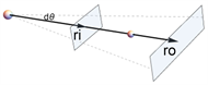
Calabi required Kahler manifolds, with the property that we can put the origin of a local coordinate system at any point, such that the metric will look like a standard Euclidean metric at that point. For simplicity, pick a point on the outer equator and choose a path that loops through the “hole” in the donut and eventually returns to the starting point. Such a path is closed. But we could have chosen a point on the equator infinitesimally close to the point we did choose, and created a new closed path in which every point on the new path is infinitesimally close to the equivalent point on the original path. One can show by construction (Figure 5(a)) that the two paths do not cross each other or intersect. The process of adding new paths infinitesimally displaced from the last path effectively builds a “sheet” of flow with surface energy density σ. Every point on the torus can be considered part of a sheet flowing up across the outer equator and down across the inner equator.

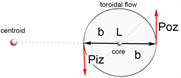
Ontologically, if we build the donut with smaller circles centered on a large circle in the plane of the donut, the tangent of the smaller circles is constant in magnitude; the flow velocity around the small circle is constant. But we cannot construct a physical torus from adjacent circles, so we must have a helical structure such that the flow is not only around the small “circle”, but also flows around the donut hole. Toroidal flow as an idealized helix leads to constant velocity, yet, ontologically, the topology is based on “surface flow”. If the surface flow along the outer equator is “up”—then continuous flow must be “down” along the inner equator of the torus. Consider a segment of arbitrary length $\Delta x_o$ and arbitrary height $\Delta y_o$ at the outer equator with flow velocity $v_o$ as seen in Figure 7(a) with the segment between the two dashed radial lines shown as a green overlay on the torus. In Figure 7(b) we show the outer segment and corresponding inner segment, extracted from the torus.

In Figure 7(a) the green segment on the outer equator of the torus is labeled with arc length $\Delta x_o$ and height $\Delta y_o$ , yielding segmental area $\Delta a_o=\Delta x_o\Delta y_o$ , through which the surface density of field energy flows with (upward) velocity $v_{oz}$ . Figure 7(b) shows both segments labeled, with the inner segment described by arc length $\Delta x_i$ and height $\Delta y_i$ yielding segmental area $\Delta a_i=\Delta x_i\Delta y_i$ with inner velocity $v_{iz}$ , flowing down across the inner equator. A U(1) slice through the torus perpendicular to both equators has two half circles, inner and outer, so we set segment heights equal, such that $\Delta y_o=\Delta y_i$ . The toroidal velocity plot, Figure 6, shows that the velocity varies from minimum to maximum, so we assume that $v_o\ne v_i$ . It is obvious that the length $\Delta x_i$ of the inner subtended arc is less than that of the outer subtended arc $\Delta x_o$ so that $\Delta x_o>\Delta x_i$ . (Similarly, lengths $\Delta y_j$ could be that of arc subtended by $\Delta \varphi$ so that $\Delta y_o>\Delta y_i$ ). With the topology and geometry of the surface flow described, we next analyze the physical ontology.

(a) (b)

Figure 7. (a) Two arbitrary radii establish two arc segments subtended by the angle between the dashed lines. A green segment of height $\Delta y_o$ spans the arc between these dashed lines. (b) The corresponding segment on the inner equator is shown from a different perspective. Surface energy density is assumed to flow through both segments. The labelled inner and outer segments are shown with respective vertical velocities $v_{iz}$ and $v_{oz}$ .

The circulating field energy density is proportional to $C\cdot C$ , where $\nabla \times C=-p$ . Although we envision the vortex surface as two dimensional, let us assume a finite wall thickness $\Delta r_j$ so that we can write the field density as volume energy density $\rho ~C\cdot C$ and mass flow (momentum $P_j$ ) through a segment with volume $\Delta x_j\Delta y_j\Delta r_j$ proportional to

$P_j=\left(\Delta x_j\Delta y_j\Delta r_j\right){\rho }_j{v}_j=$ mass flow of field through wall segment j (9)

This momentum induces more C-field circulation, as analyzed in the mass-gap existence proof; the stable final state of the topological ontological structure is assumed to represent a fermion.

A stable continuous mass flow (momentum) up through the outer segment is assumed to equal the mass flow (momentum) down through the corresponding inner segment through conservation of momentum, thus all vertical mass flow across the outer equator equals vertical mass flow across the inner equator. If we turn the torus upside down, inner flow is up and the outer down, while the meaning of inner and outer equators will not change; therefore we use equator indices {i, o}:

$v_{oz}=-v_{iz}\Rightarrow \Delta V_o{\rho }_o{v}_{oz}=-\Delta V_i{\rho }_i{v}_{iz}\Rightarrow P_{oz}=-P_{iz}$ (10)

The negative sign denotes oppositely directed vertical velocities of vertical mass flows across outer and inner equators. Assume that vertical parameters $\Delta y_j$ and wall thicknesses $\Delta r_j$ are equal, then

$\frac{\left|v_{iz}\right|}{\left|v_{oz}\right|}=\frac{{\rho }_o}{{\rho }_i}\frac{\Delta V_o}{\Delta V_i}\Rightarrow \frac{{\rho }_o}{{\rho }_i}\frac{\Delta x_o}{\Delta x_i}$ (11)

We group the energy/mass density ${\rho }_j$ with the relevant velocity $v_j$ , cancel the product of vertical parameters and wall thickness $\Delta y_i\Delta r_i=\Delta y_o\Delta r_o$ and convert horizontal parameters, the segment lengths, to arc lengths for angle $\Delta \theta$ between the dashed lines, where $0<\Delta \theta \le 2\pi$ and arc length subtended by the angle is $\Delta x_j=r_j\Delta \theta$ . Since $\Delta \theta$ cancels for all values of the angle, reduce (11) to vertical momentum density (mass density flows) $p_{iz}$ and $p_{oz}$ such that

$\frac{{\rho }_i\left|v_{iz}\right|}{{\rho }_o\left|v_{oz}\right|}=\frac{r_o}{r_i}\Rightarrow r_i{p}_{iz}=r_o{p}_{oz}=constant$ (12)

and expand the geometric product: $r_j{p}_{jz}=r_j\cdot p_{jz}+r_j\wedge p_{jz}$ . Both $j=i$ and $j=o$ radius vectors are perpendicular to the vertical momentum vectors, Figure 8, hence scalar products $r_j\cdot p_j\equiv 0$ and, converting to cross products, we have

$r_i\times p_{iz}=-r_o\times p_{oz}$ . (13)

Thus, we have coupled the density flow parameters $p_{jz}$ to the topology parameters $r_j$ . For an arbitrary slice through the torus the centroid angular momentum (point at center of hole) is:

$L_{centroid}=r_i{p}_{iz}+r_o{p}_{oz}\equiv 0$ (14)

The angular momentum of the centroid is shown to have a specific direction in the xy-plane for arbitrary $\theta$ (slice) therefore the value of $L$ must be zero. The bivector relation is $r_i{p}_{iz}=-r_o{p}_{oz}$ since vertical velocities have opposite directions with respect to the centroid, hence we have $r_i\times p_{iz}=-r_o\times p_{oz}$ . With angular momentum density of the slice measured at the centroid zero; we calculate the angular momentum density at the torus core:

$L_{core}=b\times p_{iz}+b\times p_{oz}$ (15)

Since $r_i{p}_{iz}=-r_o{p}_{oz}$ and $P_{jz}=\left({\rho }_j\Delta V_j\right)v_{jz}$ where $\Delta V_j=\Delta x_j\Delta y_j\Delta r_j$ and $\Delta x_j=r_j\Delta \theta$ with $\Delta y_j$ and $\Delta r_j$ the height and thickness of the j^th equatorial segment specified as $\Delta y_i=\Delta y_o$ and $\Delta r_i=\Delta r_o$ so that $m_j={\rho }_j\left(r_j\Delta \theta \Delta y\Delta r\right)$ under the assumption that the same mass flows across the inner and outer equatorial segments: $m_i=m_o$ . From the above:

$\frac{\left|p_{iz}\right|}{\left|p_{oz}\right|}=\frac{r_o}{r_i}=\frac{{\rho }_i}{{\rho }_o}\frac{v_{iz}}{v_{oz}}$ (16)

Based on the helical velocity the vertical velocity components are equal $v_{iz}\equiv v_{oz}$ , despite that we have shown that $v_o>v_i$ . If so, then we have

$\frac{{\rho }_i}{{\rho }_o}=\frac{r_o}{r_i}\Rightarrow {\rho }_i=\left(\frac{r_o}{r_i}\right){\rho }_o$ (17)

Figure 8. Cartoon depicting relevant vectors of the torus model of the fermion. The radii r_i, r_o, and R used in measurements in Table 1.

Thus, mass density of the inner equatorial segment is greater than the outer by ratio ( $r_o/r_i$ ) and we have arrived at a relation between the topology and the (vertical) field momentum density. We rewrite angular momentum at the core, $L_{core}=b\times P_{iz}+b\times P_{oz}$ , as

$L_{core}=b\left({\rho }_i\Delta V_i{v}_{iz}+{\rho }_o\Delta V_o{v}_{oz}\right)~b\left(m_i{v}_{iz}+m_o{v}_{oz}\right)$ (18)

Note that $b=\frac{r_o-r_i}{2}$ and that we have specified that the same mass must flow across the inner and outer equators, hence $L_{core}=\frac{r_o-r_i}{2}\left[m_i{v}_{iz}+m_o{v}_{oz}\right]$ . Since $m_i=m_o$ and $v_{iz}=v_{oz}$ the angular momentum at the core is $L_{core}=\left(\frac{r_o-r_i}{2}\right)2m_i{v}_{iz}$ or

$L_{core}=\left(r_o-r_i\right)m_j{v}_{jz}$ , (19)

where

$m_j~\underset{\text{localenergydensity}}{\underset{︸}{C\cdot C}}\underset{\text{localsegmentvolume}}{\underset{︸}{\Delta V_j}}$ (20)

and $v_{jz}$ is the vertical velocity at equator j. Angular momentum at the toroidal core is induced by energy flowing at the toroidal surface. The energy flowing at the toroidal surface is equivalently induced/sustained by the core “current”, that is, we again arrive at a relation between the topology and the field momentum density, related to the motion of the field energy density.

We conclude this section on ontological flow by observing that the velocity variations seen in Figure 6 imply that toroidal flow velocity varies and thus cannot be the constant speed of light. In other words, variations in energy density of the vector field flow through space, but NOT at the speed of light. The speed of light describes the propagation of a stress wave in the field across space.

9. Separation of U(1) × U(1) Flow Symmetry

The relevant symmetry is U(1) × U(1) and we have up to this point focused on the U(1) circulation about the torus through the donut hole and have required a constant mass flow through the hole: $p_{iz}=-p_{oz}$ . Next, we focus on the other U(1) circulation, that around the hole in the donut. In other words, the U(1) × U(1) symmetry is resolved into two orthogonal flows $p=p_z+p_{\theta }$ where $p_z$ is the momentum through the hole and $p_{\theta }$ is the momentum around the hole. Referring to Figure 8 we have three well defined radii, $r_i$ , $r_o$ and R, defining respectively the radius of the inner equator, the outer equator, and the core of the torus. Each of these distances is associated with a velocity: $\left|v_{\theta }\right|=\sqrt{v_x^2+v_y^2}$ . Whereas the vertical velocity $v_{jz}$ is constant, independent of r or θ, the mass flow through any given segment is proportional to the arc subtended by $\Delta \theta$ , and the mass of each segment, by construction, is equal to that of the other segment, independent of $\Delta \theta$ and of $\Delta y\Delta r$ , therefore the mass flow associated with each segment is proportional to $v_{j\theta }$ , i.e., $p_{j\theta }=m_j\left(r_j\right)v_{j\theta }$ . Since $v_{o\theta }>v_{i\theta }$ we have $p_{o\theta }>p_{i\theta }$ . Angular momentum $L$ at the centroid and at any point on the core are due to equatorial vertical velocities $v_{iz}=v_{oz}$ while $v_o>v_i$ . Next consider angular momentum due to corresponding horizontal components $v_{o\theta }>v_{i\theta }$ with

$v_o=v_{oz}+v_{0\theta }$ and $v_i=v_{iz}+v_{i\theta }$ . (21)

Angular momentum at the centroid due to equatorial momentum in the xy-plane is:

$L~r_i\times m_i{v}_{i\theta }+r_o\times m_o{v}_{o\theta }$ (22)

with $r_o>r_i$ and $v_{o\theta }>v_{i\theta }$ where $v_{i\theta }=\sqrt{{\left(v_{ix}\right)}^2+{\left(v_{iy}\right)}^2}$ and $v_{o\theta }=\sqrt{{\left(v_{ox}\right)}^2+{\left(v_{oy}\right)}^2}$ . We thus resolve ontological flow on the torus into two components; vertical components rotate around the core (and through the hole) and induce angular momentum in the xy-plane at the core. Horizontal components flow around the hole in the θ direction and induce angular momentum (C-field) in the z-direction at the centroid. Vertical velocities are the same value at inner and outer equators, while horizontal velocity at the outer equator is greater than that at the inner equator. Conservation of mass flow in both directions is achieved via compensating changes in local field density, with the greater density appearing at the inner equator.

However, unlike the vertical momentum, which is constant around the torus, the horizontal momentum around the hole varies with the distance from the centroid and applies to mass that is off the equatorial plane, requiring integration over all radii from $r_i$ to $r_o$ complicating the issue. For that reason, we take a different approach to the problem. Rather than attempting to calculate the horizontal momentum associated with every point on the torus, we study the third Heaviside Equation in Equation (3): $\nabla \times C=-\rho v$ derived from the primordial self-interaction Equation (1). We ignore the time change in gravity field $G$ . The $\nabla \times C$ represents the circulation of the field induced by momentum density and $\rho =\frac{\text{mass}}{\text{volume}}=\frac{m}{{\displaystyle \int {\text{d}}^{3}x}}$ with $v$ the velocity of the U(1) mass density circulation in the equatorial plane, $~C_{\theta }\cdot C_{\theta }$ . If $P$ is the momentum of this U(1) circulating field, then the U(1) circulation in the vertical plane is

$\nabla \times C=-P/{\displaystyle \int {\text{d}}^{3}x}~\left(\frac{C_{\theta }\cdot C_{\theta }}{c^2}\right)v_{\theta }$ (23)

In this case the mass density $\rho$ moving with velocity $v$ is the mass of the horizontal C-field circulation induced by the helical solenoid divided by the relevant volume, $V={\displaystyle \int {\text{d}}^{3}x}$ , that is

$\rho v=p=P/{\displaystyle \int {\text{d}}^{3}x}$ (24)

Here momentum $P$ will be identified with the core of the torus, and volume with the inside of the torus. Recall that the minus sign in Heaviside’s equation is associated with the direction of flow of the induced C-field circulation, we will drop it in our calculations of magnitude. We follow Arfken [16] and set an infinitesimal volume to be ${\displaystyle \int {\text{d}}^{3}x}=\text{d}x\text{d}y\text{d}z$ (cube) and specialize to the cylindrical volume corresponding to the U(1)-based ${\text{e}}^{iCt}$ helix, in which case we redefine the volume in cylindrical coordinates as

${\displaystyle \iiint {\text{d}}^{3}x}={\displaystyle \iint \text{d}x\text{d}y}{\displaystyle \int \text{d}z}\Rightarrow {\displaystyle {\iint }_{S}r\text{d}r\text{d}\varphi }{\displaystyle \int \text{d}z}$ (cylinder) (25)

If we integrate z from 0 to 1 the result is the unit normal ${\displaystyle {\int }_0^1\text{d}z}=\hat{n}=\frac{n}{\left|n\right|}$ to the vertical plane of circulation. We next use these results to invoke quantum half-integral spin.

10. Derivation of Quantum Spin

From the above, applying Stokes’s theorem to Heaviside’s equation $\nabla \times C=-\left(\frac{g}{c^2}\right)\rho v$ :

${\displaystyle {\iint }_S\text{d}a\hat{n}\cdot \left(\nabla \times C\right)}={\displaystyle {\oint }_{\partial S}C\cdot \text{d}l}$ (26)

we obtain the line integral around the closed (vertical) path. For a given momentum (in the z-direction) the circulation in the vertical plane is fixed and $\hat{n}\cdot \left(\nabla \times C\right)$ must not depend on the coordinate system. In the following we make use of the dimensional relations:

$\left[da\right]=l^2$ , $\left[\frac{g}{c^2}\right]=\frac{l}{m}$ , $\left[\rho \right]=\frac{m}{l^3}$ , $\left[\hat{n}\right]=1$ , $\left[v\right]=\frac{l}{t}$ , $\left[C\right]=\frac{1}{t}$ , $\left[\lambda \right]=l$ . (27)

To obtain

$\text{d}a\hat{n}\cdot \left(\nabla \times C\right)=l^2\left(\frac{l}{m}\right)\left(\frac{m}{l^3}\right)v$ (28)

where velocity $v$ is perpendicular to the plane of the C-field circulation.

The results in Equation (28) allow us to modify equation (26) as follows:

$m{\displaystyle {\iint }_S\text{d}a\hat{n}\cdot \left(\nabla \times C\right)}=mv=P=m{\displaystyle {\oint }_{\partial S}C\cdot \text{d}l}$ (29)

At this point recall that our goal is to derive a fermion from a theory of quantum gravity, so we invoke deBroglie’s fundamental basis of quantum theory, $P=\frac{h}{\lambda }$ . Substituting this into Equation (29) and multiplying both sides by $\lambda$ we obtain for $\lambda =\lambda \hat{n}$ and unit mass, $m=1$ :

${\displaystyle {\iint }_S\lambda \cdot \nabla \times C\text{d}a}=h$ (30)

This is a novel quantum relation, relating the wavelength of the core momentum to the circulation induced by this momentum and finding the quantized results in terms of Planck’s constant. Since ${\displaystyle \int {\text{d}}^{3}x}=\lambda \cdot {\displaystyle \int {\text{d}}^{2}x}$ so $\lambda$ is the length of the helical cylinder. From Equation (29) we further obtain

$m\lambda {\displaystyle {\oint }_{\partial S}C\cdot \text{d}l}=h$ , ${\displaystyle {\oint }_{\partial S}C\cdot \text{d}l}=\left(\frac{1}{m}\right)\frac{h}{\lambda }=\left|v\right|$ (31)

which implies that the circulation around a closed loop is quantized, and that it is the gauge field vector. Of course, the helix is not closed, but the torus induced by momentum $P$ is closed, and that is the focus of our next development. We have calculated the vertical contributions of the field energy density momentum to the core of the torus and the centroid of the torus. We here identify the horizontal contribution to the angular momentum as related to Planck’s constant.

11. Vector Transport around a Closed Path

Many are familiar with vector transport on the surface of a sphere—begin at the north pole and follow any longitude line to the equator, maintaining the vector as tangent to the curve at every point along the curve. When the equator is reached, the vector points south, and motion along the equator retains this direction of the vector. After reaching an arbitrary longitude begin moving the vector toward the north pole, maintaining its tangent nature at every point. When the north pole is reached, the final tangent vector is not parallel to the original vector at the same pole. The pole is used for simplicity, but this concept applies at any point and in any coordinate system. The concept of “holonomy” is a measure of how tangent vectors on a particular surface get twisted up in such parallel transport over a loop around the surface. In fact, to tie Calabi-Yau to string theory, supersymmetry was used as the bridge to holonomy; holonomy was used as the bridge to Calabi-Yau.

To analyze vector transport on the torus we arbitrarily choose the starting point on the vertical axis at R (red arrow in Figure 8). The green arrow of length b ends on the starting point. As this is at the top of the torus, the vertical coordinate is not changing at this point, hence ${\stackrel{\dot{}}{v}}_z=0$ . As we move off the starting point toward an equator, the vertical component of velocity becomes nonzero, finally reaching $v_{iz}$ (or $v_{0z}$ ) at the equator, then proceeding toward the bottom of the torus where again ${\stackrel{\dot{}}{v}}_z=0$ . Continuing this U(1)-symmetry vertical motion the point of interest is transported around the torus through the “donut hole”. But the ontological flow has U(1) × U(1) symmetry and flows around the donut hole as parameter $\theta$ increases. Therefore, when the flow crosses the inner equator the velocity at $r_i$ is $v_i=v_z+v_{\theta }$ where $v_{\theta }$ is the rotational velocity of the flow in the xy-plane. The flow of the field is left-handed with respect to the core flow. The z-component of velocity $v_{iz}$ is maximum at the equator, then diminishes until it vanishes at the bottom-most parts of the torus.

A 360˚ θ-rotation effects one complete circle around the torus, but only half a rotation about the hole in the torus; the final point on the path does not overlay the starting point. In every case, regardless of starting point, a further 2π rotation will return to the starting point, thus requiring a total 4π-rotation to close the path, as required for fermions. Once we determine that one circulation around the donut hole corresponds to two circulations around the “helical” torus, we invoke Equation (31) to conclude that 2 ${\displaystyle {\oint }_{\partial S}C\cdot \text{d}l}=h$ . This implies that the relevant wavelength is 2λ and thus, compatible with Equation (29), we have:

${\displaystyle {\iint }_S\lambda \cdot \nabla \times C\text{d}a}=\frac{h}{2}$ . (32)

That is, the quantum gravity-based spin of the fermion is $\frac{h}{2}$ . This implies, correctly as we have seen, that the C-field must wind about the torus twice to return to its starting state.

12. Measurements on a Dynamic Model

Rather than complicating the visual dynamic flow further, by dividing it into two components as it flows around the torus, I decided to also dynamically display the values of the horizontal and vertical components of velocity as it flows through every point. I typically employ 360 points for each U(1) path, and so can, via Mathematica controls, determine the speed of simulation, as it is quite simple to walk my way around the path, slowing down at each of the critical points (the red and green arrow heads in Figure 9(c)) examining the velocity components, equatorial vertical velocities $v_{iz}=v_{oz}$ with $v_o>v_i$ and corresponding horizontal components $v_{o\theta }>v_{i\theta }$ with

$v_o=v_{oz}+v_{o\theta }$ and $v_i=v_{iz}+v_{i\theta }$ . (33)

thereby building a table as seen in Table 1. The radii are defined in Figure 8, with $r_i$ the inner radius, $r_o$ the outer radius, and R the radius to the core of the torus.

At any point on the manifold the velocity $v=v_{\theta }+v_Z$ . If we square both sides, term $v_{\theta }\cdot v_Z=0$ since $v_{\theta }$ and $v_Z$ are orthogonal, hence

$v=\sqrt{v_{\theta }^2+v_Z^2}$ (34)

Table 1. Measurement of velocity components.

(a) (b) (c)

Figure 9. Based on equation 29 we draw a closed path around the torus, with the area of the enclosed xy-plane defining the horizontal boundaries of the torus. (a) shows a perspective angle on the path, while (b) shows an overhead perspective of the same path, and (c) depicts a semi-opaque torus with white outer equator shown and the closed path traversing the torus shown in black with colored arrows indicating direction of flow.

For example, at 30˚ the velocity is $\sqrt{9^2+9^2}=12.7279220$ while at 90˚ $v=\sqrt{3^2+9^2}=9.48$ . We see from the table that the measurements confirm the intuitively derived relations based on the reasoning about conservation of momentum. In short, the dynamic visualization of the field behavior intuitively confirms the correctness of the model/theory, while the measurement access to arbitrary parameters can serve as proof of the flow model worked out by conservation equations and the U(1) × U(1)-symmetry. When these measurements on the model agree in detail with intuitively and/or analytically derived behavior, the feeling is as if one has “struck gold”. One can only sincerely thank David Hestenes and Steven Wolfram for their contributions to this task.

13. Summary

There are a lot of details in this paper, and my focus has been primarily on getting the details right. An anonymous reviewer asked for more context, and this has improved the presentation of the information, for which I am grateful.

The key to fermion spin is its half-integral nature. This was first interpreted from spectral statistics, and then projected onto Stern-Gerlach beam-splitting experimental results seen in the infamous Bohr-postcard. The formulation fits the expected data, but no physical basis of half-integer spin is known. Explained succinctly, half-integral spin is not mapped into itself in one revolution, but requires a 4π-rotation, a decidedly nonclassical result. The simplest math analog is the mobius strip, but no one takes that seriously. The complete lack of ontological theory of half-integral spin has led to such explanations as Feynman’s “belt trick” wherein unobservable “tethers” are “tangled” such that a single rotation does not allow untangling to occur, while a 4π rotation untangles the system, restoring it to its initial state. Interestingly, Schiller has issued a preprint [17] based on a formalization of the belt trick.

The half-integral spin that flows from primordial field theory is not based on a belt trick; it is based on Heaviside’s gravitomagnetic dual to electromagnetism. The issue of computation of flow on the surface of the torus is one that is best addressed by constraining all calculations to the manifold defined by Calabi-Yau. This avoids any use of strings, while allowing use of Hestenes’ Geometric Calculus—instantiated in Wolfram’s Mathematica 13. The flow of C-field energy density around the surface of the torus is complicated; the vector being transferred around the path is always changing. Even the use of magnitude-adjusted, color-coded vectors is dynamically complex. A dynamically stable model of this complexity is a very strong argument for the integrity of the mathematical design. The ability to make measurements on the dynamic model which can then be compared to the predicted measurement results is rather convincing.

An Internet search for Calabi-Yau topology returns images of the type shown in Figure 10. They’re often viewed as “compactified”, meaning that the local topology exists at every point in 3D space. This is the “trick” that allows string theorists to claim that 10D and 11D theories are meaningful. A decade of operation of the LHC has failed to find any signs of supersymmetry, and string theory makes no sense without supersymmetry; nevertheless, support from the string theory community kept Calabi-Yau alive during its critical period.

Of course, in the context of today’s mysteries in physics, and ready belief in higher dimensionality at fundamental levels, such images are always enjoyed by physicists and the artistically inclined; but even if higher dimensional models turn out to be physically inappropriate, the Calabi-Yau manifolds retain supreme importance for (3D + 1)-space-time physics: they allow the use of Euclidean space tools locally in a global non-Euclidean ontology. In other words, we are allowed to compute flows on toroidal surfaces confidently.

In summary, a new theory of physics based on the existence of a primordial field at the creation of the universe resolves a number of paradoxes [logical contradictions] associated with 20th century physics. It contrasts with quantum field theory, which has one field per particle, and with general relativity, which equates the world to geometry.

Figure 10. A 10D Calabi-Yau manifold image designed by Stewart Dickson at redbubble.com.

The new theory leads almost immediately to Heaviside’s equations of gravity, dual to Maxwell’s equations of electromagnetism. While these are generally recognized as iteratively equivalent to Einstein’s field equations, physicists have been ultimately confused by the label “weak field approximation”. Primordial field equations are density-based and hold at all field strengths.

In “Self-linking Field Formalism” [18] we note that the gravitomagnetic field, induced by and inter-acting with mass flow, is significantly different from the electromagnetic field induced by and interacting with charge flow, in that the electromagnetic field is uncharged and hence cannot interact with itself. The gravitomagnetic field has energy density, hence mass density, and can therefore interact with and induce itself.

The U(1) × U(1) symmetry described herein supports two orthogonal circulations, vertical and horizontal. It seems reasonable that these self-sustaining interactions have equal angular momenta, that is, each mode supports $\frac{h}{2}$ . The vertical momenta induce the flow at the core, whereas the horizontal momentum produces the half-integral spin at the centroid. Only this spin is measurable.

Based on analogy with electromagnetism, we show that gravitomagnetism supports field structures that are self-induced; these structures include vortices in turbulent fluid, and we have shown that higher order self-interactions lead to toroidal structures that are self-stabilizing, thus bringing Calabi-Yau theory into the picture. The key contribution of Calabi-Yau to primordial field theory is found in the definition of Kahler manifold, vanishing Chern class, and Ricci-flat geometry. These establish a topological geometry framework subject to existence proofs. String theory has focused on 10D and 11D structures, for reasons to be examined elsewhere. Primordial field theory deals with (3D + 1) of space and time. We consider the torus structure to be effectively described by U(1) × U(1) symmetry, in which a 4π rotation is required to transform any point in the flow into itself via vector transport over a path on the surface of the torus. This correlates perfectly with the half-integral spin that characterizes fermions.

Analysis of the flow of the gravitomagnetic field energy density on the toroidal surface leads to formulating flow relations through the donut hole and around the donut hole, with the velocity at any point resolved into $v_z$ velocity and $v_{\theta }$ velocity.

Because primordial field theory is ontologically well defined, and the fermion is topologically well defined, we create a model fermion based in the mass-gap existence proof, now augmented by the half-integral spin existence proof. We then make measurements on this well-defined model and prove that our ontological analysis has yielded dynamical equations that match the measurements at well-defined points. This is considered an existence proof of the half-integral fermion spin.

The above theory is classical in nature, as is relativity. The quantum is introduced by invoking the key quantum relation underlying all quantum mechanics: deBroglie theorem: $p=h/\lambda$ .

14. Conclusions

The above summary reviewed the fact that our primordial field theory is now adorned with two key proofs for toroidal fermions:

· Mass-gap existence proof

· half-integral spin existence proof

Note that the standard model of particle physics has no explanation of particle mass nor any explanation for half-integral spin. Nor can it calculate the mass of any particle. Of course, at this point, primordial field theory cannot calculate fermion mass either. It is known that the C-field circulation energy has mass density, and it is also known that rotational energy is mass [19] . What has not yet been proved is the nature of electric charge in primordial field theory. We cannot nail down the mass and size of the fermion until we include the charge and associated fields, which are not assumed present at the Creation. The goal is to show that this follows from the principles of the primordial field theory.

Conflicts of Interest

The author declares no conflicts of interest regarding the publication of this paper.

References

[1]	Sbitnev, V. (2019) Foundations of Physics, 49, 107-143. https://doi.org/10.1007/s10701-019-00236-4
[2]	Klingman, E. (2022) Journal of Modern Physics, 13, 1128-1145. https://doi.org/10.4236/jmp.2022.137065
[3]	Feynman, R. (1995) Feynman Lectures on Gravitation. Westview Press, Boulder.
[4]	Armas, J. (2021) Conversations on Quantum Gravity. Cambridge University Press, Cambridge. https://doi.org/10.1017/9781316717639
[5]	Einstein, A. (1952) Relativity. Crown Publishing, New York.
[6]	Klingman, E. (2020) Journal of Modern Physics, 12, 65-81. https://doi.org/10.4236/jmp.2021.122007
[7]	Yau, S. (2010) The Shape of Inner Space. Basic Books, New York.
[8]	Heaviside, O. (1893) The Electrician, 31, 81-82.
[9]	Klingman, E. (2022) Journal of Applied Mathematics and Physics, 10, 2292-2302. https://doi.org/10.4236/jamp.2022.107156
[10]	Jaffe, A. and Witten, E. (2022) Quantum Yang-Mills Theory. https://www.claymath.org/wp-content/uploads/2022/06/yangmills.pdf
[11]	Douglas, M. (2004) Yang-Mills Existence and Mass Gap: Prove That for Any Compact Simple Gauge Group G, Quantum Yang-Mills Theory of R4. https://www.researchgate.net/publication/237610692
[12]	Klingman, E. (2022) Journal of Modern Physics, 13, 347-367. https://doi.org/10.4236/jmp.2022.134025
[13]	Klingman, E. (2021) Journal of Modern Physics, 12, 1190-1209. https://doi.org/10.4236/jmp.2021.129073
[14]	Klingman, E. (2019) Prespacetime Journal, 10, No. 6. https://prespacetime.com/index.php/pst/article/view/1602
[15]	Vishwakarma, R. (2013) Gravity of : A New Paradigm in GR. arXiv:1206.2795v2
[16]	Arfken, G. (1966) Mathematical Methods for Physicists. Academic Press, New York.
[17]	Schiller, C. (2023) Testing a Model for Emergent Spinor Wave Functions Explaining Gauge Interactions and Elementary Particles. https://www.researchgate.net/publication/361866270_Testing_a_model_for_emergent_spinor_wave_functions_explaining_gauge_interactions_and_elementary_particles
[18]	Klingman, E. (2021) Journal of Modern Physics, 12, 440-452. https://doi.org/10.4236/jmp.2021.124031
[19]	Smith, J. (2018) Physical Review Letters, 120, Article ID: 143002.