Enhancing Pneumonia Detection in Pediatric Chest X-Rays Using CGAN-Augmented Datasets and Lightweight Deep Transfer Learning Models

Coulibaly Mohamed¹, Ronald Waweru Mwangi², John M. Kihoro³

¹Department of Mathematics, Pan African University Institute for Basic Sciences, Technology and Innovation (PAUSTI), Nairobi, Kenya.
²Department of Computing, Jomo Kenyatta University of Agriculture and Technology, Nairobi, Kenya.
³School of Computing and Mathematics, The Cooperative University of Kenya, Nairobi, Kenya.

DOI: 10.4236/jdaip.2024.121001                

Abstract

Pneumonia ranks as a leading cause of mortality, particularly in children aged five and under. Detecting this disease typically requires radiologists to examine chest X-rays and report their findings to physicians, a task susceptible to human error. The application of Deep Transfer Learning (DTL) for the identification of pneumonia through chest X-rays is hindered by a shortage of available images, which has led to less than optimal DTL performance and issues with overfitting. Overfitting is characterized by a model’s learning that is too closely fitted to the training data, reducing its effectiveness on unseen data. The problem of overfitting is especially prevalent in medical image processing due to the high costs and extensive time required for image annotation, as well as the challenge of collecting substantial datasets that also respect patient privacy concerning infectious diseases such as pneumonia. To mitigate these challenges, this paper introduces the use of conditional generative adversarial networks (CGAN) to enrich the pneumonia dataset with 2690 synthesized X-ray images of the minority class, aiming to even out the dataset distribution for improved diagnostic performance. Subsequently, we applied four modified lightweight deep transfer learning models such as Xception, MobileNetV2, MobileNet, and EfficientNetB0. These models have been fine-tuned and evaluated, demonstrating remarkable detection accuracies of 99.26%, 98.23%, 97.06%, and 94.55%, respectively, across fifty epochs. The experimental results validate that the models we have proposed achieve high detection accuracy rates, with the best model reaching up to 99.26% effectiveness, outperforming other models in the diagnosis of pneumonia from X-ray images.

Keywords

Pneumonia Detection, Pediatric Radiology, CGAN (Conditional Generative Adversarial Networks), Deep Transfer Learning, Medical Image Analysis

1. Introduction

Pneumonia, primarily caused by viruses or bacteria, is a form of acute respiratory infection and a major global health concern affecting all age groups. It is particularly deadly for children, being the single largest infectious cause of death worldwide in this demographic. In 2017 alone, pneumonia claimed the lives of over 808,000 children under the age of five, representing 15% of all deaths in this age group. The disease significantly impacts the lungs’ alveoli, small sacs crucial for oxygen exchange. In pneumonia, these alveoli fill with pus and fluid, making breathing painful and limiting oxygen intake, thus severely affecting respiratory function. The transmission of pneumonia typically occurs through direct contact with infected individuals. This alarming prevalence underscores the urgent need for effective detection and treatment strategies, especially in vulnerable populations and regions with limited healthcare infrastructure [1] [2] [3] . The importance of early detection and timely treatment is paramount to prevent the progression to more severe, potentially fatal stages.

The convergence of robust computing systems and sophisticated algorithms has revolutionized the healthcare landscape, introducing a new epoch where the automation of diagnostic processes that traditionally depended on the expertise of medical professionals has become a reality [4] . Artificial intelligence (AI), particularly in the form of deep convolutional Neural Networks (D-CNN), is reshaping the field of medical imaging. While it does not seek to replace human experts, it serves as a powerful tool to assist in complex diagnoses, often surpassing human capabilities in both speed and accuracy [5] . The advent of deep learning and advancements in deep convolutional neural networks has brought the practice of transfer learning to the forefront. Leveraging the weights of CNNs pre-trained on extensive datasets such as ImageNet, this method has become a cornerstone in medical imaging research, especially where datasets are inherently limited in size [6] . The promise of D-CNN in diagnosing, detecting, classifying, and segmenting pneumonia from medical images has garnered significant interest, given the demonstrated success of these networks in medical image analysis [3] .

Despite the advancements in healthcare technology, pneumonia diagnosis remains a challenge. The integration of AI and D-CNN in medical imaging has opened new possibilities for automated diagnosis. However, this approach faces significant challenges, such as limited and imbalanced datasets, and a discrepancy between the characteristics of natural images used in pre-training and those of medical images. These issues hinder the effective application of deep learning in medical diagnostics, particularly for pneumonia, where accurate and timely detection is critical [6] . Addressing these hurdles requires innovative solutions, such as fine-tuning pre-trained networks on specialized datasets to improve performance, a method that can offer substantial benefits over building models from scratch [4] .

Our research aims to address the challenges of data scarcity and model effectiveness in the AI-driven diagnosis of pneumonia. By implementing Conditional Generative Adversarial Networks (CGAN), we intend to enrich the quality and quantity of data for underrepresented classes, overcoming the obstacle of limited training data. Furthermore, we plan to deploy and evaluate a series of lightweight Deep Transfer Learning (DTL) models, aiming to achieve exceptional diagnostic accuracy. This approach is expected to underscore the transformative potential of AI in medical imaging and demonstrate the critical role of fine-tuned, lightweight neural networks in the detection and diagnosis of pneumonia.

2. Related Works

2.1. Automated Diagnosis of Pneumonia Using CNN and Transfer Learning Approaches

This study [2] proposes a deep learning system for automated diagnosis of pneumonia using chest X-ray images. The authors identify the images as normal or pneumonia patients using CNN and transfer learning algorithms. The study’s dataset is made up of chest X-rays from children and women in Guangzhou. According to the results, the transfer learning model, especially the XceptionNet model, had the best accuracy of 93%. However, the ensemble model, which includes three separate models, performed better overall, but with somewhat lower accuracy. The suggested system has the potential to improve pneumonia identification and treatment. However, the research makes no mention of potential biases in the dataset used to train the deep learning models, which might impair the generalizability of the results. Furthermore, the study does not investigate the interpretability of deep learning models, which is critical for understanding how these algorithms make decisions.

2.2. A Comparison of Deep CNN Architectures for Pneumonia Detection

In their research, [3] introduced an automated approach for distinguishing between bacterial and viral pneumonia using digital chest X-ray images. A comparative analysis was carried out on various CNN architectures such as VGG19, ResNet152v2, Resnext101, Seresnet152, Mobilenettv2, and DenseNets with 201 layers. Among these, DenseNets emerged as the most efficient, registering a test accuracy of 95%. To enhance model performance, transfer learning and ensemble techniques were incorporated. This study underscores the proficiency of deep CNNs in pneumonia diagnosis and emphasizes the significance of prompt detection for improved patient prognosis. However, it is critical to recognize the research’s limitations. The use of a small dataset and dependence on free resources may have limited the scope and depth of the studies, thus affecting their generalizability and robustness.

2.3. Deep Transfer Learning Model with Classical Data Augmentation and CGAN for COVID-19 Detection from Chest CT Radiography Images

The authors suggested a deep transfer learning model with conventional data augmentation and conditional generative adversarial networks (CGAN) for COVID-19 identification from chest CT radiography images in this study [7] . The authors overcome the limitations of the COVID-19 CT datasets by using data augmentation methods and CGAN to produce extra training images. To identify the CT images, several deep convolutional neural network (DCNN) architectures were used, including AlexNet, VGGNet16, VGGNet19, GoogleNet, and ResNet50. The findings show that the ResNet50 model detects COVID-19 with the best accuracy from the enhanced dataset. The combination of data augmentation methods with CGAN enhances dataset size and improves deep transfer learning model performance. The work emphasizes the significance of early COVID-19 identification as well as the prospective uses of GANs and CGANs in picture production and unsupervised learning. The study paper’s disadvantage is the lack of a rigorous examination of the suggested DTL models on a bigger and more varied dataset to determine their generalizability.

2.4. Classification of Diseases from X-Ray Images Using Conditional Generative Adversarial Networks and Transfer Learning

This paper examines illness categorization using X-ray images, including COVID-19, pneumonia, and tuberculosis [8] . It presents a model for exact categorization that combines a Conditional Generative Adversarial Network (CGAN) with fine-tuned deep transfer learning. To balance the dataset, CGAN is used to generate additional training images. Pre-processing approaches such as histogram equalization and lung segmentation improve image quality. Using the augmented images, many pre-trained models, including ResNet-50, ResNet-101, and others, are modified. The results show that incorporating produced images improves model accuracy during training, validation, and testing. Some constraints of the study may have an impact on the model’s performance. The use of a small and unbalanced dataset, which may not be reflective of the actual world, is one restriction. Another issue is that the CGAN-generated images are lower resolution than the original dataset images, which may make extracting features from the images challenging for the model. Furthermore, differences in the settings and characteristics of the chest X-ray images may induce biases in the categorization findings. Finally, when the model is applied to a test dataset that is not the same as the training and validation datasets, its accuracy may suffer.

2.5. Deep Transfer Learning

A significant challenge in training deep learning models is the lack of substantial quantities of labeled medical images. In the early stages of the COVID-19 pandemic or even a year after its onset, obtaining ample labeled chest X-ray data for deep learning training remained a hurdle [9] . To address this, numerous studies have adopted transfer learning, leveraging knowledge from CNN models trained on vast image datasets like ImageNet [4] .

Transfer learning can be categorized from two perspectives: feature space and label space. Based on these perspectives, it can be classified into homogenous and heterogenous transfer learning. For instance, when comparing solely based on image data, a dataset of X-ray images might be viewed as heterogeneous in relation to a dataset of tree species pictures. However, when the comparison encompasses both audio and text datasets, the X-ray dataset might be seen as homogeneous to the tree species picture dataset. Additionally, based on label-setting criteria, DTLs can be divided into three types: 1) transductive, 2) inductive, and 3) unsupervised. In simpler terms, transductive refers to cases where only the source data has labels, inductive is when both source and target data possess labels, and when neither datasets are labeled, it’s termed as unsupervised deep transfer learning [9] .

A single CNN model comprises various convolutional, pooling layers and others. These layers are responsible for extracting features from images or videos, with the deeper layers capturing more intricate deep features [7] . The initial layers of the model are either fixed or fine-tuned, while the latter layers are trained specifically on the target dataset [4] .

Consider the layer l of a convolutional layer. If we have a square grid of neuron nodes with dimensions $N\times N$ , followed by a convolutional layer, and then apply a filter with dimensions $M\times M$ represented as W, the resulting output from the convolutional layer will have dimensions $\left(N-M+1\right)\times \left(N-M+1\right)$ , generating k feature maps [7] . The dot product is computed by the convolutional layer by taking its input and multiplying it by the filter weights, as illustrated in Figure 1. The convolutional layer acts as a feature detector, detecting properties in its inputs. Before adding nonlinearity, this layer recognizes visual characteristics such as edges, lines, and corners to compute the input. The input for layer $l\times 1$ is supplied as follows 1:

$Z_i^l=B_i^l+{\displaystyle \underset{a=1}{\overset{N}{\sum }}}{\displaystyle \underset{b=1}{\overset{N}{\sum }}}{W}^i{X}_{\left(i+a\right)\left(j+b\right)}^{l-1}$ (1)

where $B_i^l$ indicates a bias value matrix and $W_i$ means a masking matrix with dimensions $M\times M$ . Following that, the convolutional layer employs the activation function defined in Equation (2).

Figure 1. Convolutional and pooling layers producing feature maps. (a) convolutional layer; (b) pooling layer.

$\text{Net}=r\left(Z_i^l\right)$ (2)

where r(.) is a function that introduces nonlinearity, which is essential in Deep Transfer Learning methods. Several functions, including the hyperbolic tangent (tanh), sigmoid function, and rectified linear units (ReLU), can be used for this purpose. In our technique, the ReLU and sigmoid function are used as the activation function in Equations (3) and (4). This option is chosen to expedite the learning process. The ReLU and function are defined by the expression:

$r\left(u\right)=\max \left(0,u\right)$ (3)

Which outputs either the input value if it’s positive, or zero if it’s not.

$f\left(x\right)={\left(1+{\text{e}}^{-x}\right)}^{-1}$ (4)

The sigmoid function creates an S-shaped curve by gradually transitioning values from near-zero to near-one.

3. Methodology

3.1. Dataset Description

The whole dataset included 5858 chest X-ray images, 1584 normal images, and 4274 pneumonia images. The dataset is divided into three folders: train, test, and val, with subfolders for each image category (Pneumonia/Normal). The full dataset was obtained using kaggle from retrospective cohorts of pediatric children aged one to five years old at Guangzhou Women and Children’s Medical Center in Guangzhou. The dataset was highly skewed and constrained. [8] .

3.2. Proposed Model

The proposed framework consists of two main components. The first component utilizes CGAN for data augmentation, while the second component integrates four individual lightweight DTL models as shown in Figure 2. CGAN is primarily used in the preprocessing phase to generate synthetic data, while DTL is used in the performance measurement phase to train and evaluate models.

Algorithm 1 delineates the framework for a Deep Transfer Learning strategy tailored to classify chest X-ray images into two distinct categories, namely NORMAL and PNEUMONIA. The approach leverages a collection of efficient lightweight DTL architectures including MobileNet, MobileNetV2, Xception, and EfficientNetB0, denoted by $M$ .

These models undergo a meticulous tuning process with a dataset $\left(X_{\text{input}}\mathrm{,}{y}_{\text{input}}\right)$ , where $X_{\text{input}}$ constitutes a series of N images each with a resolution of 224 × 224 pixels, and $y_{\text{input}}$ consists of the associated categorical labels within the set {NORMAL, PNEUMONIA}.

Figure 2. The suggested architecture employs CGAN and lightweight DTL models.

Algorithm 1. Suggested Lightweight DTL Model based on CGAN for Chest X-ray Classification.

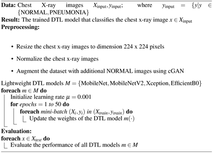
The learning rate $\lambda$ , a critical tuning parameter, is employed to adjust the models’ weights during the training phase. This phase is structured into three segments: a training set $\left(X_{\text{train}}\mathrm{,}{y}_{\text{train}}\right)$ , a validation set $\left(X_{\text{val}}\mathrm{,}{y}_{\text{val}}\right)$ , and a test set $\left(X_{\text{test}}\mathrm{,}{y}_{\text{test}}\right)$ . The training set is subdivided into mini-batches of size 64,

represented as $\left(X_i\mathrm{,}{y}_i\right)\in \left(X_{\text{train}}\mathrm{,}{y}_{\text{train}}\right)$ for $i=\mathrm{1,2,}\cdots \mathrm{,}\frac{N}{64}$ , and is iteratively used

to fine-tune the Lightweight DTL models, denoted as $d\in D$ , to minimize empirical loss, characterized by Equation (5):

$L\left(w\mathrm{<mo>\; ;\; </mo>}{X}_i\right)=\frac{1}{n}{\displaystyle \underset{\left(x\mathrm{,}y\right)\in \left(X_i\mathrm{,}{y}_i\right)}{\sum }}\mathcal{l}\left(m\left(x\mathrm{,}w\right)\mathrm{,}y\right)$ (5)

In this case, $\mathcal{l}(\cdot )$ is the binary cross-entropy loss function, and $m\left(x\mathrm{,}w\right)$ is the DTL prediction function that assesses the likelihood of class y for an input x, given the set of weights w.

3.3. A Conditional Generative Adversarial Network

A conditional GANs are a type of GAN that takes in additional information to help the generator and discriminator learn. This information could be the class of the current image or some other property [10] . Generative models produce new instances influenced by the input data provided. Like other deep neural networks used for image creation, GANs produce images that align with the distribution of the input images [8] while CGANs incorporate two distinct networks (the generator and the discriminator) that utilize a conditional label as shown in 3 [7] . The generator within the CGAN deceives the discriminator by producing images that appear real. Conversely, the discriminator network aims to discern between genuine and generated images. The models undergo adversarial training, where a reduction in the generator’s loss correlates with an increase in the discriminator’s loss, and vice versa.

In the generator, the initial input noise $p_z\left(z\right)$ and y are integrated into a shared hidden layer. The design of the adversarial training setup offers ample leeway in shaping this hidden layer. In the discriminator, both x and y are used as inputs to a differentiation function [11] .

Two losses need to be computed for the Discriminator: one associated with the “fake” image and the other with the “real” image. Their sum constitutes the comprehensive loss for the Discriminator. Consequently, the Discriminator’s loss function is designed to minimize the discrepancy in predictions for real images obtained from the dataset and fake images produced by the Generator, all while taking their one-hot labels into account.

Discriminator’s loss function is shown in 6

$L_D=-V\left(D\mathrm{,}G\right)=-{\mathbb{E}}_{x~p_{\text{data}}\left(x\right)}\left[\log D\left(x\mathrm{<mo>\; |\; </mo>}y\right)\right]-{\mathbb{E}}_{z~p_z\left(z\right)}\left[\log \left(1-D\left(G\left(z\mathrm{<mo>\; |\; </mo>}y\right)\right)\right)\right]$ (6)

And the loss function of the generator minimizes the correct prediction of the discriminator on fake images conditioned on the specified one-hot labels.

$L_G=-{\mathbb{E}}_{z~p_z\left(z\right)}\left[\log D\left(G\left(z\mathrm{<mo>\; |\; </mo>}y\right)\right)\right]$ (7)

Finally, the objective function for a two-player minimax game can be represented as shown in 8 [11] .

$\underset{G}{\min }\underset{D}{\max }V\left(D\mathrm{,}G\right)={\mathbb{E}}_{x~p_{\text{data}}\left(x\right)}\left[\log D\left(x\mathrm{<mo>\; |\; </mo>}y\right)\right]+{\mathbb{E}}_{z~p_z\left(z\right)}\left[\log \left(1-D\left(G\left(z\mathrm{<mo>\; |\; </mo>}y\right)\right)\right)\right]$ (8)

This Equation (8) represents a two-player minimax game where the generator (G) tries to minimize the function, and the discriminator (D) tries to maximize it.

Where:

Ÿ $D\left(x\mathrm{<mo>\; |\; </mo>}y\right)$ : denotes the discriminator estimated probability for the sample of real data.

Ÿ (x): is the actual reality for class (y).

Ÿ $D\left(G\left(z\mathrm{<mo>\; |\; </mo>}y\right)\right)$ : denotes the discriminator estimated probability for the sample of fake data.

The CGAN architecture and its constituent layers can be summarized as (Figure 3):

1) Generative network:

Ÿ 2—Input Layers

Ÿ 2—Dense Layers

Ÿ 1—Embedding Layer

Ÿ 5—Conv2DTranspose Layers (Convolutional Layer with upsampling)

Ÿ 1—Conv2D Layer (Convolutional Layer with downsampling)

Ÿ 5—Leaky ReLu

2) Discriminator Network:

Ÿ 2—Input Layers

Ÿ 2—Dense Layers

Ÿ 1—Embedding Layer

Ÿ 5—Conv2D Layer (Convolutional Layer with downsampling)

Ÿ 1—Dropout Layer

Ÿ 5—Leaky ReLu

Once the discriminator and generator networks were established, we trained the model over 250 epochs. During this training, the discriminator’s loss for real images fluctuated between 0.3 and 0.6, just as the loss for fake images did. However, for the majority of the training duration, the generator’s loss remained slightly above 1. After trained, the generative network is then used to generate the synthetic images of the normal class in order to balance the data sets.

Figure 3. Conditional generative adversarial network model.

Figure 4 present the samples from original and generated X-ray images of normal lung conditions. Using a generative network, the images in section B were synthesized to mimic those in section A. Upon visual inspection, the generated images closely resemble their original counterparts, highlighting the capability of the generative model.

First Figure 5 displays an initial dataset with a class imbalance with a lower count of “NORMAL” (blue bar) compared to “PNEUMONIA” (red bar) while the second 6 shows the dataset after employing CGAN to synthesize images for the “NORMAL” class, achieving an equal number of samples for both classes, thus rectifying the imbalance and facilitating the training of more accurate and unbiased diagnostic models (Figure 6).

Figure 4. Conditional generative adversarial network model. (a) Original normal images; (b) Generated normal images.

Figure 5. Initial data distribution across the classes.

Figure 6. Data distribution after applied cGAN technique.

4. Experiments

4.1. Dataset Splitting

During the partitioning process, we divide the dataset into two segments. The initial segment, constituting 70% of the dataset, is reserved for training purposes. The remaining 30% is allocated for both testing and validation. The count of divided images with CGAN enhancement is detailed in Table 1. The original dataset contained 5217 images for training, 16 images for validation, and 625 images for testing. After augmenting the dataset with CGAN-generated images, the number of images increased significantly. The training set grew to 5982 images, the validation set to 1709 images, and the testing set to 855 images.

4.2. Experimental Setup

The experiments were conducted using Tensor Flow version 2.9.1 and were trained on the PaperSpace cloud platform, which includes an Ampere A4000, 8 CPUs, 45 GB of RAM, and a 16 GB GPU.

4.3. Training Parameter Settings

The pre-trained models underwent training for 50 epochs, utilizing shuffled mini-batches comprising 64 images each. Adam optimizer was employed with a learning rate set at 0.001, and binary cross-entropy was used as the loss function. Additional elements integrated into the network layers included a flattening layer, two dropout layers with dropout probabilities of 0.2 and 0.5, respectively, and a batch normalization layer, with the sigmoid function serving as the classifier. A dense layer with 64 neurons is used in all the models following the first dropout layer, which has a dropout probability of 0.2.

Table 2 provides a detailed breakdown of the parameters used in various Deep Transfer Learning architectures, emphasizing their optimization settings.

Table 1. Distribution of chest X-ray pneumonia images in the original and CGAN enhanced dataset.

Table 2. Configuration parameters of DTL models.

4.4. Light Weight Pre-Trained Models Architectures

Training a neural network from the ground up requires a substantial amount of data. However, with transfer learning, a smaller training dataset can be utilized to produce a precise and extensive set of features. Given that the majority of chest x-ray pneumonia datasets are relatively small, due to medical ethical standards, privacy considerations and the expenses associated with their creation, it takes longer to develop a proficient model. Consequently, the suggested models are based on lightweight pre-trained architectures and are tailored to classify pneumonia instances.

4.4.1. MobileNet

The MobileNet architecture employs depth-wise separable convolutions, positioning it as a lightweight model [12] . It introduces two global hyper-parameters, allowing developers to select the appropriate model size for their specific use case. MobileNet is both trained and evaluated on ImageNet for the purpose of image classification.

To reduce computational costs, MobileNet employs Depth-wise separable convolution and point-wise convolution instead of standard convolution [13] . This approach aims to minimize the number of Floating Point Operations Per Second (FLOPS) and Multi-Add operations, as detailed in Figure 7.

Figure 7. Depth-wise separable convolution and point-wise convolution. (a) Standard Convolution Filters; (b) Depthwise Convolutional Filters.

4.4.2. MobileNetV2

MobileNetV2 represents an enhancement over the original MobileNet design, demonstrating top-tier performance across various tasks and benchmarks [12] . The primary contribution lies in the introduction of a new layer module, the inverted residual with linear bottleneck. This module accepts a low-dimensional compressed representation as input. Initially, the input is expanded to a higher dimension and then filtered using a lightweight depthwise convolution. Subsequently, the features are projected back to a low-dimensional representation via a linear convolution. A notable modification is the elimination of non-linearities in the narrow layers to preserve representational power [13] . Within the inverted residual block, the intermediate layers undergo an expansion, effectively thickening them. This expansion, despite increasing the number of filters in these intermediate layers, actually reduces computational costs by decreasing the number of input and output channels, as illustrated in Figure 8. The architecture is trained and evaluated for both object detection and image classification tasks.

4.4.3. Xception

The Xception network incorporates depth-wise separable convolution layers. It is designed to map both spatial and cross-channel correlations, which can be fully disentangled in CNN feature maps [14] . While it retains the foundational structure of Inception, the Xception model has 36 convolution layers, which can be grouped into 14 distinct modules. Excluding the initial and final layers, each layer possesses a consistent residual connection around it. The model processes the input image by transforming spatial correlations to attain cross-channel correlations within each output channel. A full depiction of the network’s specifications is illustrated in Figure 9.

4.4.4. EfficientNetB0

The EfficientNetB0 series, a recent family of architectural designs, has demonstrated remarkable performance superiority in classification tasks compared to other networks, all while maintaining a lower parameter count and computational load (FLOPs) [12] . It adopts a technique known as compound scaling, which efficiently and uniformly adjusts the network’s width, depth, and resolution, as demonstrated in Figure 10. This innovation leads to EfficientNet models

Figure 8. (a) Residual block; (b) Inverted residual block.

Figure 9. Architecture of the xception model showing entry, middle, and exit flows.

Figure 10. Model Scaling. (a) is a baseline network example; (b)-(d) are conventional scaling that only increases one dimension of the network width, depth, or resolution. (e) is our proposed compound scaling method that uniformly scales all three dimensions with a fixed ratio.

having parameters that are 8.4 times smaller and achieving 6.1 times faster inference speeds when compared to the best-performing existing networks. The EfficientNet family includes multiple versions, ranging from B0 to B7. The choice of which EfficientNet model to use can be made based on available computational resources and cost considerations. For instance, EfficientNet-B0 consists of 5.3 million parameters, whereas the most recent iteration, EfficientNet-B7, boasts a larger model with 66 million parameters.

4.5. Evaluation Criteria

Various performance metrics are employed to evaluate the effectiveness of machine learning classification models based on CNN algorithms. These metrics include accuracy (AC), precision, recall, F1-score, and the confusion matrix (CM).

4.5.1. Accuracy

This metric evaluates the total number of instances correctly predicted by the trained model relative to all possible instances. Accuracy is defined as the proportion of images accurately classified to the total number of images provided.

$Accuracy=\frac{TP+TN}{TP+TN+FP+FN}$ , (9)

where TP refers to true positive, TN refers to true negative, FP refers to false positive, and FN refers to false negative values.

4.5.2. Precision

This metric measures the proportion of true positive cases among all predicted positive instances. For instance, in the context of pneumonia, it represents how accurately the model identifies patients with pneumonia. Precision becomes a pertinent measure when false positives carry more significance than false negatives. It is mathematically represented as follows:

$Precision=\frac{TP}{TP+FP}$ , (10)

where TP refers to true positive and FP refers to false positive values.

4.5.3. Recall

This metric assesses the model’s ability to correctly detect pneumonia patients out of all actual cases of pneumonia. Recall becomes an important measure when the consequences of false negatives outweigh those of false positives. It is defined mathematically by the subsequent equation:

$Recall=\frac{TP}{TP+FN}$ , (11)

where TP refers to true positives and FN refers to false negative values.

4.5.4. F1-Score

The F1 score offers a combined metric of classification accuracy, taking into account both precision and recall. It is the harmonic mean of the two, providing a balance between them. The F1 score reaches its maximum value when precision and recall are equal. This measure effectively gauges the model’s comprehensive performance by integrating the results of both precision and recall.

$F_1\text{Score}=\frac{2\times \text{Precision}\times \text{Recall}}{\text{Precision}+\text{Recall}}$ (12)

The training loss measures the model’s performance on the training dataset, while the validation loss gauges its performance on unseen data. Essentially, a loss value indicates the efficiency of a predictor in categorizing the provided data. The better the model is at capturing the relationship between input data and its intended output, the smaller the loss. Nevertheless, there’s a threshold to how accurately we can fit the training data, beyond which our model may compromise its ability to generalize.

4.5.5. Confusion Matrix (CM)

A confusion matrix presents algorithm performance in a tabular format. It offers a visual representation of key predictive metrics like recall, specificity, accuracy, and precision. Through the CM, values like TP, FP, TN, and FN can be straightforwardly compared. The term “support” refers to the occurrences of the desired class within the dataset. If there’s an imbalance in support in the training data, it could highlight potential vulnerabilities in the classifier’s scores, suggesting the possible need for measures like stratified sampling or rebalancing.

5. Result Analysis and Discussion

We look at the performance characteristics of four popular lightweight DTL models in this section: MobileNet, MobileNetV2, Xception, and EfficientB0. We begin by displaying their categorization results 3. Following that, a complete examination of their overall findings without and with CGAN is shown in Tables 4-6.

The performance of four fine-tuned lightweight architectures is discussed in this section. As indicated in Table 3, the models MobileNet, MobileNetV2, Xception, and EfficientNetB0 all achieved high accuracy scores on the aggregated test dataset. The test accuracies were determined by the ratio of correctly identified samples to the total samples. The Xception model stood out with an accuracy of 99.26%. Noteworthy is the enhancement in accuracy for the MobileNet, MobileNetV2, and EfficientNetB0 networks from their initial configuration to after fine-tuning.

Table 4 shows the accuracy of each DTL model on the test set. The results are divided into two training scenarios: first, using only original data, and second, using the original data augmented with synthetic chest X-ray images generated by a CGAN. The accuracy statistics from the table are impressive. They show that using CGAN-generated data significantly improves the performance of DTL models. For example, the MobileNet model’s accuracy increases from 61.37% when trained on the original data to 92.94% when trained on the CGAN-augmented

Table 3. Training, validation and testing binary accuracy for models trained with the help of generated images.

Xception and MobileNetV2 showed highest training and testing acuracy while MobileNet and MobileNetV2 showed highest validation accuracy.

Table 4. DTL testing accuracy for the both scenarios.

data. Similar improvements are observed for MobileNetV2, Xception, and EfficientNetB0, with all models demonstrating significant accuracy gains when trained on the enriched dataset.

The recall rates in Table 5 show how challenging the original dataset is, with MobileNet achieving a recall rate of only 38.46%. This is significantly improved to 98.46% by adding CGAN data. This improvement is important because it suggests that augmenting training with CGAN images can greatly reduce the number of false negatives. This is vital in clinical settings to ensure that all cases of a condition are identified. MobileNetV2 and EfficientNetB0 exhibited perfect recall with both original and CGAN-augmented datasets, reflecting their strong generalization abilities. Despite the original data’s imbalance, these models demonstrated high recall, suggesting they could learn to identify minority class instances effectively. Xception also maintained high recall across datasets, indicating its robust performance in class imbalance conditions and confirming its reliability for tasks requiring high recall. The precision metrics for models, as shown in Table 6, provide insights into the models’ performance in classifying positive instances correctly when trained on different datasets. MobileNet’s precision decreased slightly when supplemented with CGAN-generated images, dropping from 99.33% to 90.99%. In contrast, the precision for MobileNetV2, Xception, and EfficientNetB0 increased when trained on the augmented dataset. The rise from 62.5% to 88.43% for MobileNetV2 and from 62.5% to 93.31% for EfficientNetB0 is particularly noteworthy, indicating a significant benefit from the inclusion of CGAN data. Xception’s precision increase to 97.66% underscores its capability to maintain high precision despite the increased dataset complexity.

Table 5. Testing recall for the both scenarios.

Table 6. Testing precision for the both scenarios.

The precision improvements with CGAN-augmented data suggest that some models benefit from the extended feature set of synthetic images. Additionally, the varying impact of CGAN on different model architectures indicates that a model’s structure may affect its adaptability to enhanced data diversity.

The training times for the DTL models MobileNet, MobileNetV2, Xception, and EfficientNetB0 are comparable, as evidenced by their similar total training times (MobileNet: 10389.02 seconds, MobileNetV2: 10494.16 seconds). This consistency in training times indicates that these models exhibit comparable efficiency during the training process.

The significant boost in model accuracy, achieved through data augmentation using CGAN, emphasizes its capability in mitigating the constraints posed by limited datasets. Expanding the dataset by generating more images for both labels further reinforces this approach. This advancement opens avenues for further exploration, particularly in customizing CGAN to cater to a variety of medical imaging applications. One promising area of development is the enhancement of the CGAN architecture itself, possibly by adding more layers for more sophisticated data processing. Figure 4, which contrasts original and CGAN-generated images for the NORMAL label, highlights a current limitation: the lower resolution of generated images compared to their original counterparts. Addressing this by generating higher-resolution images could substantially enhance model performance, as higher resolution would allow the model to discern and utilize more detailed features. Additionally, the impressive performance metrics observed suggest the importance of real-world validation. Future research should prioritize testing these models on larger and more diverse datasets, which is essential to confirm the models’ robustness and practical effectiveness in real-world medical settings.

5.1. Detailed Performance Metrics of Fine-Tuned DTL Models

Tables 7-10 provide a detailed breakdown of the performance metrics (precision, recall, F1-score, and support) for four different DTL models that were fine-tuned for a classification task involving chest X-ray images. These metrics are crucial for validating the effectiveness of the models in distinguishing between “Normal” and “Pneumonia” conditions on the original testing set.

Table 7. Precision, recall and F1-score result of fine-tuned MobileNet.

Table 8. Precision, recall and F1-score result of fine-tuned MobileNetV2.

Table 9. Precision, recall and F1-score result of fine-tuned Xception.

Table 10. Precision, recall and F1-score result of fine-tuned EfficientNetB0.

Table 7-10 presents the precision, recall, F1-score, and specificity results for the lightweight networks with fine-tuning applied. Typically, a model that exhibits high precision, recall, and support is deemed better. Based on the table’s data, all four models successfully detected pneumonia.

5.2. Training and Validation Binary Accuracy and Loss of Fine Tuning DTL Models

Figures 11-14 illustrate the training and validation accuracy of the fine-tuned models. The x-axis denotes the number of epochs, while the y-axis indicates the percentages for accuracy and loss.

Figure 11. Training and validation accuracy and loss over the epochs (Fine-tuned MobileNet Network).

Figure 12. Training and validation accuracy and loss over the epochs (Fine-tuned MobileNetV2 Network).

Figure 13. Training and validation accuracy and loss over the epochs (Fine-tuned Xception Network).

In DCNN, a loss function is utilized to refine the architecture. The loss is computed using both training and validation datasets, with the cumulative performance in these datasets indicating the model’s effectiveness. Essentially, the loss equates to the cumulative errors attributed to every sample in the training or validation sets. The loss value after each iteration signifies the effectiveness of a model’s performance.

5.3. Confusion Matrix after Fine-Tuned DTL Models

The confusion matrix is a performance metric that provides more insights into the achieved testing accuracy. Figures 15-18 illustrate the confusion matrices for two classes of DTL models with the help of CGAN.

Figure 14. Training and validation accuracy and loss over the epochs (Fine-tuned EfficientNetB0 Network).

Figure 15. CM of fine-tuned MobileNet.

Figure 16. CM of fine-tuned MobileNetV2.

Figure 17. CM of fine-tuned Xception.

Figure 18. CM of fine-tuned EfficientNetB0.

6. Conclusion

Recognizing the critical importance of timely and precise diagnosis, this research contributes to significantly advancing the detection of pneumonia in children under five, a demographic particularly vulnerable to this life-threatening condition. Pneumonia infection is diagnosed using medical images, including chest X-ray images. The primary issue with medical images is the small dataset available for training Deep Learning models. To tackle the limited dataset issue, the CGAN technique was adjusted to produce more realistic images, thereby achieving a balanced dataset. This dataset contains 8548 chest X-ray images distributed across two classes. With augmentation, the dataset reached a size conducive for effective training and the generation of dependable outcomes. Such enrichment of the dataset enabled deep transfer learning models like MobileNet, MobileNetV2, Xception, and EfficientB0 to diagnose pneumonia with high efficiency. Further examination of these models’ performance revealed that, notably, the Xception model attained an accuracy exceeding 99.26% consistently across 50 epochs. This result underscores the model’s superior performance when trained on an augmented dataset, enhancing overall diagnostic metrics.

Conflicts of Interest

The authors declare no conflicts of interest regarding the publication of this paper.

References

[1]	WHO (2023) Pneumonia. https://www.who.int/health-topics/pneumonia/#tab=tab_1
[2]	Madhavi, A., Abhijna, M.S., Sumanjali, P., Supraja, S., Ghalwan, M. and Chary, M.R. (2023) Automated Diagnosis of Pneumonia Using CNN and Transfer Learning Approaches. E3S Web of Conferences, 430, 01031. https://doi.org/10.1051/e3sconf/202343001031
[3]	Porag, A.M.R., Hasan, M.M. and Ahad, M.T. (2022) A Comparison Study of Deep CNN Architecture in Detecting of Pneumonia. arXiv Preprint arXiv:2212.14744.
[4]	Mukhlif, A.A., Al-Khateeb, B. and Mohammed, M.A. (2022) An Extensive Review of State-of-the-Art Transfer Learning Techniques Used in Medical Imaging: Open Issues and Challenges. Journal of Intelligent Systems, 31, 1085-1111. https://doi.org/10.1515/jisys-2022-0198
[5]	Masud, M. (2022) A Light-Weight Convolutional Neural Network Architecture for Classification of COVID-19 Chest X-Ray Images. Multimedia Systems, 28, 1165-1174. https://doi.org/10.1007/s00530-021-00857-8
[6]	Wen, Y., Chen, L., Deng, Y. and Zhou, C. (2021) Rethinking Pre-Training on Medical Imaging. Journal of Visual Communication and Image Representation, 78, 103145. https://doi.org/10.1016/j.jvcir.2021.103145
[7]	Loey, M., Manogaran, G. and Khalifa, N.E.M. (2020) A Deep Transfer Learning Model with Classical Data Augmentation and CGAN to Detect COVID-19 from Chest Ct radiography Digital Images. Neural Computing and Applications, 1-13. https://doi.org/10.1007/s00521-020-05437-x
[8]	Mehta, T. and Mehendale, N. (2021) Classification of X-Ray Images into COVID-19, Pneumonia, and TB Using CGAN and Fine-Tuned Deep Transfer Learning Models. Research on Biomedical Engineering, 37, 803-813. https://doi.org/10.1007/s42600-021-00174-z
[9]	Iman, M., Arabnia, H.R. and Rasheed, K. (2023) A Review of Deep Transfer Learning and Recent Advancements. Technologies, 11, Article 40. https://doi.org/10.3390/technologies11020040
[10]	Nayak, M. (2018) An Introduction to Conditional GANS (CGANs). Medium.
[11]	Mirza, M. and Osindero, S. (2014) Conditional Generative Adversarial Nets. arXiv Preprint arXiv:1411.1784.
[12]	Elharrouss, O., Akbari, Y., Almaadeed, N. and Al-Maadeed, S. (2022) Backbones-Review: Feature Extraction Networks for Deep Learning and Deep Reinforcement Learning Approaches. arXiv Preprint arXiv:2206.08016.
[13]	Zhu, F. (2021, January 22) MobileNets, EfficientNet and EfficientDet. https://seventt.github.io/2021/01/22/model-efficiency-and-model-accuracy/
[14]	Kathamuthu, N.D., Subramaniam, S., Le, Q.H., Muthusamy, S., Panchal, H., Sundararajan, S.C.M., Alrubaie, A.J. and Zahra, M.M.A. (2023) A Deep Transfer Learning-Based Convolution Neural Network Model for COVID-19 Detection Using Computed Tomography Scan Images for Medical Applications. Advances in Engineering Software, 175, Article 103317. https://doi.org/10.1016/j.advengsoft.2022.103317