Chemical Characterization of Lake Togbadji

Vitalique Elegbede¹, Dominique Kpadonou², Joël Dossou-Gbete¹, Magloire Acakpo Nonvignon Gbaguidi², Bienvenu Olatundji Ogoudele¹

¹Doctoral School of Exact and Applied Sciences, University of Abomey-Calavi (UAC), Abomey-Calavi, Benin.
²Ecotoxicology and Quality Study Research Unit, Applied Chemistry Study and Research Laboratory, Department of Chemical Engineering-Processes (GC-P), Polytechnic School of Abomey-Calavi, University of Abomey-Calavi, Abomey-Calavi, Benin.

DOI: 10.4236/jwarp.2023.1512039                

Abstract

The present study focused on the chemical characterization of the watercourse of the Togbadji Lake wildlife ranch. The methodological approach followed is as follows: Bibliography review, Sampling campaign. The results obtained were the subject of descriptive statistics, the two-sample Wilcoxon test to determine the impact of different localities on the abundance of microbiological contaminants, a Principal Component Analysis (PCA) with the software R version 3.5.0, in order to group the pollution parameters according to the different levels and sources of contamination. From our results, it is found that the respective average values in dry and rainy seasons for ammonium ions are 0.38 ± 0.16 mg/L and 0.22 ± 0.03 mg/L; for nitrite ions 0.20 ± 0.25 mg/L and 0.02 ± 0.01 mg/L; for nitrate ions 3.72 ± 2.52 mg/L and 7.84 ± 4.91 mg/L; for total Kjeldahl nitrogen 1.27 ± 1.44 mg/L and 1.19 ± 1.49 mg/L; for orthophosphate ions 0.20 ± 0.25 mg/L and 0.02 ± 0.01 mg/L; for total phosphorus 0.04 ± 0.01 mg/L and 0.11 ± 0.23 mg/L; the chemical oxygen demand 93.36 ± 61.73 mg/L of O2 and 89.93 ± 66.11 mg/L of O2 and the biochemical oxygen demand over 5 days 25.50 ± 18.22 mg/L of O2 and 37 ± 33.15 of O2. It emerged that the main sources of pollution in Lake Togbadji are runoff water, discharges of various wastewater from artisanal activities, livestock farming and open defecation.

Keywords

Chemical Degradation, Aquatic Environment, Lake Togbadji

1. Introduction

Water is a precious natural resource essential to the life and socio-economic development of people. It is unevenly distributed across the surface of the globe. In certain places on earth, access to water resources is very difficult because of its geolocation and/or reservoir rocks. Added to this unequal distribution are the threats of alteration of water resources. They are threatened by both natural and anthropogenic processes [1] . As threats, we can cite landslides, volcanism, storms, the chemical quality of reservoir rocks, agriculture, industry, crafts, population growth, transport, poor management of waste, destruction natural resources, animal and human health care establishments, etc. [2] . Relying on the purifying properties of natural environments, man has always entrusted the environment with the free function of eliminating or keeping away the undesirables he rejects [3] . This irresponsible behavior has made the availability and especially the quality of water resources the most strategic issues of our time. If in the past the natural and/or anthropogenic microbiological degradation of natural water resources was and remains a concern, today with the development of science, techniques and technologies, chemical pollution has been added to microbiological pollution and complicates benefits the management of the quality of water resources. The physicochemical and/or microbiological alteration of natural waters has consequences both on the water resources themselves and on the populations dependent on these water resources. The findings reveal that industrial, agricultural and artisanal pollution are the most significant and the most threatening in the least developed countries [4] . Benin has a diversity of humid ecosystems resulting in the presence of a large hydrographic network unevenly distributed throughout the national territory. This network is made up of numerous rivers, lakes, lagoons and water reservoirs [5] . Like the global observation, Benin’s water resources are also exposed to natural and anthropogenic threats. With a view to preserving these aquatic ecosystems and the environmental, socio-economic and health well-being of populations, it is very important to take stock of the pollution of Benin’s waterways and bodies of water. Several studies are being carried out in this direction on a good number of water resources in Benin, especially the most important and/or strategic ones, but there are still plans and watercourses for which very few studies have been carried out as is the case for example of Lake Togbadji, of which physicochemical and/or microbiological pollution is suspected due to periodic massive deaths of unresolved fish, the last episode of which was recorded in the month of November 2021. However, we must indisputably reduce the anthropogenic pressure on hydrosystems especially in this new context of climate change which complicates the threats weighing on water resources through more pronounced episodes of drought and flooding. This approach must be informed by a diagnosis of the state of the situation which involves evaluating the levels of contamination of the water resources concerned. It is therefore fundamental to have a good understanding of the dangers and to better quantify the risks in order to be able to better set ambitious objectives for prevention, protection and appropriate management of water resources and dependent ecosystems. It is within this framework that the present study falls, the objective is to evaluate the level of chemical pollution of the aquatic ecosystem of Lake Togbadji, in the south of Benin.

2. Methodology

Study Zone

Located in the southwest of Benin, precisely in the Mono delta, Lake Togbadji is a vast expanse of stagnant water with an area of approximately 9.1509 km² and a depth ranging from 4 m to 14 m. It is located between latitude 6˚44'36 north and longitude 1˚42'9 east and near the localities of Agbodranfo, Adrogbodji, Adjakomey, Bakpohoué, Kpolédji, Takon and Togbadji. With a sword shape oriented south-north, it is a natural water source shared by the communes of Dogbo and Lokossa in the departments of Mono and Couffo. Lake Togbadji constitutes the main source of water for the Ayomi district in the commune of Dogbo. It is one of the most important lakes on the periphery of the alluvial valley of the Mono and Sazué basin characterized by a degraded and complex hydrographic network. It is fed by runoff water coming from several horizons. Figure 1 shows the study area.

3. Material and Methods

3.1. Literature Review

The documentary research consisted of browsing articles, dissertations and theses on the internet and in libraries dealing with the physico-chemical and microbiological pollution of bodies of water and courses, its environmental and health impacts, research and dosage techniques parameters for monitoring the quality of natural waters based on environmental matrices. This literature review allowed us to deepen our knowledge of our theme and to clearly understand all its contours.

3.2. Prospective Visits

Prospective field visits allowed us to familiarize ourselves with the realities of the sampling areas. Two prospective visits (one in the dry season and one in the rainy season) were organized to identify sampling sites and target groups to survey. We also took advantage of this field visit to raise awareness among local residents about the work to be carried out in order to obtain their support for the continuation of the work.

3.3. Sampling Campaigns

There are four sampling campaigns, taken twice each year, one in the dry season and one in the rainy season. All water samples were collected in previously emptied 1.5 L plastic bottles of mineral water, soaped without detergent, rinsed with tap water and then three times with distilled water. Before any sampling, the bottles thus conditioned are rinsed three times with the water to be sampled. Samples are collected in duplicate in the water column approximately 10 cm from the surface. After sampling, the bottles are labeled and stored in a cooler equipped with a cold accumulator and sent to the laboratory for analysis.

Figure 1. Location map of Lake Togbadji (Source: This study).

3.4. Laboratory Analysis

In the laboratory, the water samples are kept at 4˚C in the refrigerator until the analyzes start to slow down the degradation of the samples. The standardized methods for determining the different parameters are recorded in Table 1.

4. Results and Discussion

4.1. Results

4.1.1. Description of Parameters in Rainy and Dry Seasons

From Table 2, it appears that the content of ammonium ${\text{NH}}_{\text{4}}^{+}$ ions varies

Table 1. Standardized methods used for parameter determination.

(Source: This study).

Table 2. Description of the chemical parameters of the waters of Lake Togbadji in the dry season.

(Source: This study).

from 0.16 to 0.75 mg/L with an average of 0.383 ± 0.15 mg/L equivalent to 0.244 ± 0.095 mg/L of N. The % CV = 39.8 ≥ 30. The measured values of ammonium ions are scattered and the average is not representative of the series. Nitrite ${\text{NO}}_{\text{2}}^{-}$ ions oscillate between 0.012 and 0.10 mg/L with an average of 0.08 ± 0.028 mg/L equivalent to 0.024 ± 0.0085 mg/L of N. The %CV = 34.8. Like ammonium ions, the values taken by nitrite ions at the sampling sites are dispersed. Nitrate ions ${\text{NO}}_{\text{3}}^{-}$ vary from 1.18 to 7.6 mg/L with an average of 3.72 ± 2.43 mg/L or 0.84 ± 0.55 mg/L of N. The coefficient of variation % CV = 65.3. The values taken by the series are scattered. Total Kjeldahl NTK nitrogen ranges between 0.25 and 5.75 mg/L with a mean of 1.77 ± 1.39 mg/L and %CV = 108.8. Nitrogen pollution in general varies from one site to another on Lake Togbadji and is less than 12 mg/L of N recommended in Belgium. The orthophosphate and total phosphorus contents vary respectively between 0.085 and 1.05 mg/L with an average of 0.2 ± 0.237 mg/L with a %CV of 118.3 and between 0.02 and 0.065 mg/L for an average of 0.04 ± 0.012 mg/L with a %CV = 31.1. As in the case of nitrogen pollution, phosphorus pollution is also dispersed on Lake Togbadji, but less than 1 mg/L of P recommended for surface waters. The chemical oxygen demand (COD) on the body of water varies from 7 to 225 mg/L of oxygen with an average of 93.36 ± 59.48 mg/L and a %CV of 67.7. Although the COD value varies from one site to another on Lake Togbadji, at several sampling points the COD values are well above the recommended limit in Brussels which is 30 mg/L. The Biochemical Oxygen Demand in 5 days (BOD5) is between 4 and 58.5 mg/L for an average of 25.5 ± 17.56 mg/L and a %CV = 68.9. Like the COD, the BOD5 is also dispersed on Lake Togbadji and at several monitoring points this BOD5 takes values higher than the maximum recommended limit for surface water in Brussels which is 6 mg/L.

From the analysis of the data in Table 3, we note that in the rainy season the

Table 3. Description of the chemical parameters of Lake Togbadji in the rainy season.

(Source: This study).

content of ammonium ${\text{NH}}_{\text{4}}^{+}$ ions vary from 0.155 to 0.245 mg/L with an average of 0.215 ± 0.03 mg/L equivalent to 0.137 ± 0.019 mg/L of N. The %CV = 12.6. The measured values of ammonium ions are homogeneous and the average is representative of the series unlike in the dry season. Nitrite ${\text{NO}}_{\text{2}}^{-}$ ions vary from 0.006 to 0.031 mg/L with an average of 0.018 ± 0.006 mg/L equivalent to 0.0055 ± 0.0018 mg/L of N. The %CV = 31.6. As in the dry season, the values taken by nitrite ions at the sampling sites are dispersed. Nitrate ions ${\text{NO}}_{\text{3}}^{-}$ vary from 3.5 to 19.7 mg/L with an average of 7.84 ± 4.73 mg/L or 1.77 ± 1.07 mg/L of N. The coefficient of variation % CV = 60.4. The values taken by nitrate ions at the sampling sites are scattered. Total nitrogen Kjeldahl NTK ranges between 0.2 and 5.75 mg/L with a mean of 1.94 ± 1.43 mg/L and %CV = 120.1. Nitrogen pollution apart from ${\text{NH}}_{\text{4}}^{+}$ ions varies from one site to another on Lake Togbadji and is less than 12 mg/L of N recommended in Belgium. The orthophosphate and total phosphorus contents vary respectively from 0.012 to 0.035 mg/L with an average of 0.02 ± 0.006 mg/L with a %CV of 29.3 and between 0.025 and 0.915 mg/L for an average of 0.114 ± 0.223 mg/L with a %CV = 196.3. As in the dry season, phosphorus pollution is also dispersed on Lake Togbadji, but less than 1 mg/L of P recommended for surface waters. The chemical oxygen demand (COD) on Lake Togbadji ranges from 7 to 225 mg/L of oxygen with an average of 89.93 ± 63.71 mg/L and a %CV of 70.8. The COD as in the dry season varies from one site to another on Lake Togbadji. At several sampling points the COD values are well above the recommended limit in Brussels which is 30 mg/L. The Biochemical Oxygen Demand in 5 days (BOD5) is between 4 and 81 mg/L for an average of 37 ± 31.95 mg/L and a %CV = 86.4. Like the COD, the BOD5 is also dispersed on Lake Togbadji and at several monitoring points this BOD5 takes values higher than the maximum recommended limit for surface water in Brussels which is 6 mg/L.

4.1.2. Comparative Analysis of Chemical Parameters in Dry and Rainy Seasons

· Case of Ammonium ions

Analysis of the information recorded in Figure 2 reveals a p-value less than 0.05. Therefore, there is a significant difference between the average values of ammonium ion contents in the dry season and in the rainy season. In the rainy season the average is 0.22 ± 0.03 mg/L with a %CV of 13.07 less than 30% so in the rainy season the average ammonium ion content is representative of the series. On the other hand, in the dry season the average is 0.38 ± 0.16 mg/L with a %CV of 41.28. The average is not representative of the series. Therefore the ammonium ion contents are dispersed on Lake Togbadji in the dry season. This observation can be justified by a stratification of the lake water in the dry season and the measurements were not made at the same depth.

The seasonal distribution maps of ammonium ion contents on Lake Togbadji are presented in Plate 1. The analysis of the information on the maps reveals a north/south distribution of the observed ammonium ion contents on the lake,

Figure 2. Comparison of seasonal averages of ammonium ion contents (Source: This study).

which leads us to suspect a spatial autocorrelation of ammonium ion contents.

From the analysis of the values taken by the Moran indices, it appears that in the dry season the Moran index is different from 0, which leads to the conclusion that in the dry season the realization of the regionalized random variable is dependent. It is therefore possible to predict the ammonium ion content values at one point, knowing the values observed at another point, based on the distance which separates them in the dry season. On the other hand, in the rainy season the Moran index is close to 0, the regionalized random variable is therefore independent. It is therefore not possible to predict the ammonium ion content values at one point, knowing the values observed at another point, based on the distance which separates them in the rainy season. However, the dependence observed in the dry season and the independence of the data observed in the rainy season may be the result of chance. It is therefore necessary to verify the validity of this spatial dependence on a global scale. This statistical test of independence of the regionalized variable gives a Z score equal to 0.001 with a p-value of 0.41 in dry season while in rainy season a Z score equals 0.001 with a p-value of 0.03. Given the p-values obtained for the different seasons (p-value greater than 5% in the dry season and less than 5% in the rainy season), this test puts the interpretation of the Moran index into perspective and indicates on the one hand the non-existence in the dry season of spatial correlation on a global scale and on the other hand the existence of aggregates in the rainy season in which local autocorrelation is expressed. It is therefore appropriate to identify these aggregates in the rainy season and to look for the factors behind these concentrations of similar values at certain points. In order to locate these spatial subsets, the local spatial association indices of Anselin Local Moran and Gi* of

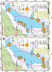
Plate 1. Spatio-temporal variation of ammonium ion contents in the waters of Lake Togbadji during the two seasons (Source: This study). (a) Distribution of ammonium ion contents in the dry season; (b) distribution of ammonium ion contents in the rainy season.

Getis-Ord are used.

4.1.3. Local Configuration of Ammonium Ion Contents According to the Anselin Local Moran Index

The Z score values of the Anselin Local Moran index were categorized into three classes. The low value class (−2.09 to −1.07) and the medium value class (−1.06 to 0.08) express a dissimilarity between neighboring points or even an average similarity. The class of strong values (0.09 to 1.71) expresses a strong similarity between neighboring points. The analysis of Figure 3 reveals that sites SL2 and SL6 in the center-east of Lake Togbadji constitute an aggregate of low Z score

Figure 3. Local configuration of ammonium ion contents according to the Anselin Local Moran index (Source: This study).

values. This area reflects a low similarity between the ammonium ion values observed at the 14 sampling points. On sites SL8, SL10, SL12 and SL13 in the southwest, site SL3 in the center-east and site SL7 north of Lake Togbadji, an aggregate of average Z score values is observed. While the sites SL1, SL4, SL5, SL11 in the center-east and SL14 in the center-west, constitute an aggregate of strong Z-score value. The central and southern areas are heterogeneous with a mixture of high, medium and low Z-score sites in the central-east, and medium and high Z-score sites in the south. This implies that the ammonium ion content values observed in these places are dissimilar.

In order to refine the clustering trends of ammonium ion content values in the study area in the rainy season and to identify areas of high concentration (hot pot) and areas of low ammonium ion concentrations, we used the Gi* from Getis-Ord. The maps in Figure 4 and Figure 5 show the spatial distributions of hot pot areas in the dry season and in the rainy season. The classification of GI* Z scores is made into three classes at the natural Jenks threshold.

4.1.4. Local Configuration According to Getis-Ord Gi* Index

Three areas emerge when observing this map. Zone 1: SL8, SL9, SL10, SL11, SL12 and SL13 constitutes an aggregate of medium and strong Z scores (average Z score between −1.03 and 1.02 and strong Z-scores between 0.19 and 0.87) south of Lake Togbadji. This zone is therefore characterized by high and medium values of ammonium ion content. The low and average Z scores are observed in zone 2 which is located in the central part of the body of water. This zone is made up of an aggregate of low values and medium values of ammonium ion content. Zone 3 is located north of the lake with a high Z score site SL7. In this zone the values of the ammonium ion content are high. The hypothesis of the existence of a structure in the spatial distribution of ammonium ion content values is therefore verified. There are concentration aggregates of high and low values as well as an orientation in the spatial distribution of ammonium ion content values in the rainy season. This observed distribution is therefore not the result of chance.

Figure 5 shows the distribution map of ammonium ion contents. Analysis of the map information reveals 5 classes of ammonium ion concentration in the study area. It’s about:

- class 1 consisting of low ammonium ion concentrations between 0.193 and 0.209 mg/L in light grenadine color;

- class 2: ammonium ion contents between 0.21 and 0.217 mg/L slightly dark grenadine color;

- class 3: ammonium ion contents between 0.218 and 0.224 mg/L dark grenadine color;

- class 4: ammonium ion contents between 0.225 and 0.232 mg/L darker grenadine color;

- class 5: ammonium ion contents between 0.233 and 0.241 mg/L very dark grenadine color;

Figure 4. Local configuration according to the Getis-Ord Gi* index.

We note that the northern part of the lake is the most contaminated with ammonium ions in the rainy season followed by the central part of the lake.

· Case of Nitrite ions

Figure 6 presents the comparison of seasonal average nitrite ion contents in the waters of Lake Togbadji. Analysis of the information recorded in the Figure shows that the p-value is less than alpha = 0.05. Therefore, there is a significant difference between the average nitrite ion in the rainy season and that of the dry season. The average in the rainy season is 0.02 ± 0.01 mg/L with a %CV of 30.45 and that of the dry season is 0.20 ± 0.25 mg/L with a %CV of 122.73. Both in the dry season and in the rainy season, the averages are not representative of the

Figure 5. Mapping of the spatial distribution of ammonium ion contents.

series. In other words, the measured values of nitrite ion contents are dispersed in the study area. Plate 2 presents the seasonal distribution of nitrite ion contents in the waters of Lake Togbadji. Analysis of the map data shows a north/south oriented distribution of nitrite content values, which raises suspicion of the existence of a spatial autocorrelation of nitrite content data. The search for the existence of autocorrelation was carried out with the statistics of Moran and General G.

Analysis of the data shows that the Moran index is close to 0, which leads to the conclusion that the realization of the regionalized random variable is therefore independent. It is therefore not possible to predict the nitrite ion content values at one point, knowing the values observed at another point, based on the

Figure 6. Comparison of seasonal averages of nitrite ion contents (Source: This study).

distance which separates them. This observed independence may be the result of chance and/or linked to the size of the sample used for the calculations. It is therefore necessary to verify the validity of this spatial independence on a global scale. The statistical test of independence of the regionalized variable gives a Z score equal to −0.827975 confirming the interpretation of the Moran index and indicates the non-existence in the dry season of spatial correlation on a global scale. What happens to these trends in the rainy season? The calculation of the spatial autocorrelation index carried out on the 14 collection points and the values observed on these points present the following results: Moran’s spatial autocorrelation index = 0.568283; Expected index = −0.076923; Variance = 0.031935; Z Score = 3.610480; p-value = 0.000306. The Moran index is different from 0, which leads to the conclusion that the realization of the regionalized random variable is therefore dependent. It is therefore possible to predict the values of the nitrite ion content at one point, knowing the values observed at another point, based on the distance which separates them. This observed dependence may be the result of chance and/or linked to the size of the sample used for the calculations. It is therefore necessary to verify the validity of this spatial dependence on a global scale. This statistical test of independence of the regionalized variable gives a p-value of 0.006935 less than alpha = 0.05, which confirms the interpretation. The Getis-Ord statistic gives Observed General G: 0.001231; General G expected: 0.001130; Variance: 0.000000; Z-score: 0.916539 and p-value: 0.359384 greater than alpha = 0.05. So the existence of a structure in the spatial distribution of Pt values is therefore not verified. There are no concentration aggregates of high and low values in the rainy season. This observed distribution is therefore the result of chance.

· Case of nitrate ions

Figure 7 presents the results of the comparison of seasonal averages of nitrate

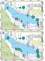
Plate 2. Spatio-temporal variation of nitrite ion contents in the waters of Lake Togbadji during the two seasons (Source: this study). (a) Distribution of nitrite ion contents in the dry season; (b) distribution of nitrite ion contents in rainy season.

Figure 7. Comparison of seasonal averages of nitrate ion contents (Source: this study).

ion contents. From the analysis of the information recorded in the Figure, it appears that the p-value is equal to 0.010 less than alpha = 0.05. Hence the difference between the means is significant. The average in the dry season is 3.72 ± 2.52 mg/L with a %CV = 67.81. By that of the wet seasons is 7.84 ± 4.91 mg/L with a %CV = 62.66. The values taken by the %CV show that the nitrate ion contents both in the dry season and in the rainy season are dispersed. Each level of nitrate ion contamination is characteristic of its observation zone, in other words the activities carried out on said site.

The maps in Plate 3 present the seasonal spatial distributions of nitrate ion contents.

Analysis of the information on the maps in Plate 3 shows that the nitrate ion content data follow a north/south direction. We deduce from this the existence of a direction in the distribution of temperature values. This allows us to suspect a spatial dependence of temperature values in the dry season, hence the need to test spatial autocorrelation.

The calculation of the spatial autocorrelation index was carried out on the 14 collection points. From the analysis of the data, it appears that in the dry season, the Moran index is close to 0, which leads to the conclusion that the realization of the regionalized random variable is therefore independent. It is therefore not possible to predict the nitrate ion content values at one point, knowing the values observed at another point, based on the distance which separates them. This observed independence cannot be the result of chance in the sense that the p-value of this statistic is equal to 0.257688 greater than alpha = 0.05. It is therefore not necessary to verify the validity of this spatial dependence on a global scale.

Let’s observe these trends in the rainy season. The values observed on these points present the following results: Moran’s spatial autocorrelation index = 0.045722; Expected index = −0.076923; Variance = 0.023748; Z Score = 0.795851; p-value = 0.426119. The Moran index is close to 0, which leads to the conclusion that the realization of the regionalized random variable is therefore independent. It is therefore not possible to predict the values of nitrate ion contents at one

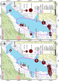
Plate 3. Spatio-temporal variation of nitrate ion contents in the waters of Lake Togbadji during the two seasons (Source: this study). (a) Distribution of nitrate ion contents in the dry season; (b) distribution of nitrate ion contents in the rainy season.

point, knowing the values observed at another point, based on the distance which separates them. This observed independence may be the result of chance and/or linked to the size of the sample. It is therefore necessary to verify the validity of this spatial independence on a global scale. This statistical test of independence of the regionalized variable gives a Z score equal to 1.018895. This Z score confirms the interpretation of the Moran index and indicates the non-existence of spatial correlation on a global scale in the rainy season.

· Case of total nitrogen Kéjdahl (NTK)

Figure 8 presents the results of comparison of seasonal averages in NTK in the waters of Lake Togbadji. The analysis of the two histograms reveals that there is not a significant difference between the seasonal means in NTK because the p-value is greater than alpha = 0.05. Likewise, the values of the standard deviations are high and by extension the coefficients of variation. The values taken by these averages are respectively 1.27 ± 1.44 mg/L with a %CV = 112.96 and 1.19 ± 1.49 mg/L with a %CV = 124.62. This observation leads us to conclude that the NTK contents observed in the waters of Lake Togbadji are dispersed. So each NTK value translates information specific to its environment. The maps in Plate 4 present the spatio-temporal distribution of NTK contents.

Analysis of the information on the maps in Plate 4 reveals a north/south orientation of NTK contents on Lake Togbadji. This observation makes it possible to deduce the existence of a direction in the distribution of NTK values allowing us to suspect a spatial dependence of NTK values in the dry season, hence the need to test spatial autocorrelation. The calculation of the spatial autocorrelation index carried out on the 14 collection points in the dry season and the values observed on these points gives a Moran index close to 0, which leads to

Figure 8. Results of the comparison of seasonal averages of NTK contents (Source: This study).

Plate 4. Spatio-temporal variation of NTK contents in the waters of Lake Togbadji during the two seasons (Source: This study). (a) Distribution of NTK contents in the dry season; (b) distribution of NTK contents in rainy season.

the conclusion that the realization of the regionalized random variable is therefore independent. It is therefore not possible to predict the NTK values at one point, knowing the values observed at another point, based on the distance that separates them. This observed independence may be the result of chance and/or the size of the sample used for the calculations. It is therefore necessary to verify the validity of this spatial independence on a global scale. This statistical test of independence of the regionalized variable gives a Z score equal to 0.963444. This Z score confirms the interpretation of the Moran index and indicates the non-existence of spatial correlation on a global scale in the dry season.

The calculation of the spatial autocorrelation index carried out on the 14 collection points in the rainy season and the values observed on these points gives a Moran index close to 0, which leads to the conclusion that the realization of the regionalized random variable is therefore independent. It is therefore not possible to predict the NTK values at one point, knowing the values observed at another point, based on the distance that separates them. Calculation of the concentration index of high values and low values of Getis-Ord General G gives the following results: Observed General G = 0.001437; Expected General G = 0.001130; General G Variance = 0.000000 and Z Score = 0.946007. According to these statistics, there are, in the dry season, aggregates in which high and low values of NTK content are concentrated.

· Case of the Orthophosphate ion

From the analysis of the data in Figure 9, it appears that the p-value = 0.011 is less than alpha = 0.05. This value of the p-value of the means comparison tests allows us to conclude that the two means are significantly different. The values taken by the averages are 0.20 ± 0.25 mg/L with a coefficient of variation %CV =

Figure 9. Comparison of seasonal averages of orthophosphate ion contents (Source: This study).

122.73 in the dry season and 0.02 ± 0.01 mg/L with a %CV = 30.45. Therefore, the orthophosphate contents observed on Lake Togbadji are dispersed around seasonal averages. The maps on Plate 5 present the seasonal distribution of orthophosphate contents on Lake Togbadji. From the analysis of these maps, we see that the direction ellipse is stretched on the north/south axis. We deduce from this the existence of a direction in the distribution of orthophosphate content values. This allows us to suspect a spatial dependence of seasonal orthophosphate values, hence the need to test spatial autocorrelation.

L’Moran index is close to 0 and allows us to conclude that the realization of the regionalized random variable is therefore independent. This observed independence may be the result of chance. It is therefore necessary to verify the validity of this spatial independence on a global scale. This statistical test of independence of the regionalized variable gives a Z score equal to 1.418292. This Z score confirms the non-existence of spatial correlation on a global scale in the dry season.

The calculation of the concentration index of high values and low values of Getis-Ord confirms the non-existence, in the dry season, of aggregates in which high values and low values of orthophosphate contents are concentrated. What happens to these trends in the rainy season?

Moran’s Spatial Autocorrelation Index is close to 0, which leads to the conclusion that the realization of the regionalized random variable is therefore independent. It is therefore necessary to verify the validity of this spatial independence on a global scale. This statistical test of independence of the regionalized variable gives a Z score equal to 0.147272 and a p-value of 0.882918. This Z score and this p-value confirm the interpretation of the Moran index and indicate the non-existence of spatial correlation on a global scale in the rainy season.

Calculation of the concentration index of high values and low values of Getis-Ord General G, gives a General G obtained = 0.001364; a Z-Score = 0.87054 and a p-value of 0.384005. According to these statistics, he does not exist, in the dry season, aggregates in which the high and low values of the orthophosphate ion content are concentrated.

· Case of total phosphorus

Figure 10 presents the results of comparison of seasonal means of total phosphorus (Pt). From the analysis of these results it appears that the p-value is greater than alpha = 0.05. So there is not a statistically significant difference between the two seasonal averages of total phosphorus. The values taken by these averages are respectively 0.04 ± 0.01 mg/L of Pt in the dry season with a coefficient of variation %CV = 32.24 and 0.11 ± 0.23 mg/L of Pt with a %CV = 203.73 in rainy season. The averages are not representative of the series and the observed Pt values are scattered both in the dry season and in the rainy season, which leads us to conclude that total phosphorus (Pt) contamination levels on Lake Togbadji depend on the sampling points. The maps in Plate 6 present the spatio-temporal distribution of Pt contents on Lake Togbadji.

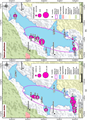
Plate 5. Spatio-temporal variation of orthophosphate contents in the waters of Lake Togbadji during the two seasons (Source: This study). (a) Distribution of orthophosphate contents in the dry season; (b) distribution of orthophosphate contents in the rainy season.

Figure 10. Comparison of seasonal averages of total phosphorus (Source: This study).

Considering the information recorded on the maps, it appears that the total phosphorus (Pt) content data observed on Lake Togbadji follow a north/south direction and leads to the conclusion of a spatial dependence of the values of total phosphorus (Pt) in all seasons, hence the need to test spatial autocorrelation. The results of the calculations of the spatial autocorrelation index were carried out on the 14 collection points.

Moran’s spatial autocorrelation index is close to 0; which leads to the conclusion that the realization of the regionalized random variable is therefore independent. It is therefore not possible to predict the total phosphorus values at one point, knowing the values observed at another point, based on the distance that separates them. This observed independence may be the result of chance and/or linked to the size of the sample used for the calculations. It is therefore necessary to verify the validity of this spatial independence on a global scale. This statistical test of independence of the regionalized variable gives a Z score equal to 1.922358 and a p-value of 0.054561. This p-value and this Z score confirm the interpretation of the Moran index and indicate the non-existence of spatial correlation on a global scale in the dry season. Calculation of the concentration index of high values and low values of Getis-Ord General G, gives an observed General G = 0.000401; an expected General G = 0.001130; General G Variance = 0.000000 and a Z Score = −1.812055 and a p-value of 0.069978. According to these statistics, there are, not in the dry season, aggregates in which high and low values of total phosphorus content are concentrated. What happens to these trends in the rainy season?

The Index Moran’s spatial autocorrelation is close to 0 also in the rainy season, which leads to the conclusion that the realization of the regionalized random variable is therefore independent. It is therefore not possible to predict the

Plate 6. Spatio-temporal variation of total phosphorus (Pt) contents in the waters of Lake Togbadji during the two seasons (Source: This study). (a) Distribution of total phosphorus (Pt) contents in the dry season; (b) distribution of total phosphorus (Pt) contents in the rainy season.

total phosphorus values at a point in the rainy season, knowing the values observed at another point, based on the distance that separates them. This observed independence may be the result of chance and/or linked to the size of the sample used for the calculations. It is therefore necessary to verify the validity of this spatial independence on a global scale. This statistical test of independence of the regionalized variable gives a Z score equal to 0.581345 and a p-value greater than alpha = 0.05. This confirms the interpretation of the Moran index and indicates the non-existence of spatial correlation on a global scale in the dry season. The calculation of the concentration index of strong values and weak values of Getis-Ord General G gives a p-value of 0.953020. According to these statistics, there do not exist, not in the rainy season, aggregates in which the high and low values of the total phosphorus content are concentrated.

· Case of Biochemical Demand in 5 days (BOD5)

The analysis of Figure 11 shows a p-value greater than alpha = 0.05, indicating that the seasonal means of BOD5 are not significantly different. The values taken by the seasonal averages are respectively 25.50 ± 18.22 mg/L of oxygen with a coefficient of variation %CV = 71.45 in the dry season. On the other hand, in the rainy season the seasonal average is 37 ± 33.15 O₂ with a %CV = 89.62. It is concluded that the BOD5 values in the waters of Lake Togbadji are scattered around the averages whatever the season. This observation reveals a diversity of intensity of biodegradable organic pollution and/or sources of pollution around Lake Togbadji. The proximity and demographics of the riverside localities seem to corroborate this assertion. The maps in Plate 7 present the seasonal distributions of the intensity of biodegradable organic pollution.

From the analysis of the information contained in the cards, it appears that

Figure 11. Comparison of seasonal averages of BOD5 (Source: This study).

Plate 7. Spatio-temporal variation of BOD5 contents in the waters of Lake Togbadji during the two seasons (Source: This study). (a) Distribution of BOD5 contents in the dry season; (b) distribution of BOD5 contents in rainy season.

the distributions of BOD5 values in the study environment in the dry season and in the rainy season follow a north/south axis. This allows us to suspect a spatial dependence of BOD5 contents, hence the need to test spatial autocorrelation. The calculation of the spatial autocorrelation index carried out on the 14 collection points in the dry season and the values observed on these points present a Moran index different from 0, which leads to the conclusion that the realization of the regionalized random variable is therefore dependent. It is therefore possible to predict the BOD5 values at one point, knowing the values observed at another point, based on the distance that separates them. This observed dependence may be the result of chance. It is therefore necessary to verify the validity of this spatial dependence on a global scale. This statistical test of independence of the regionalized variable gives a Z score equal to −0.381940 and a p-value of 0.702506. This p-value invalidates the interpretation of the Moran index and indicates the non-existence of spatial correlation on a global scale in the dry season.

The calculation of the concentration index of strong values and weak values of Getis-Ord General G, confirms the non-existence, in the dry season, aggregates in which the high and low BOD5 values are concentrated. What happens to these trends in the rainy season?

The results of the calculation of the spatial autocorrelation index carried out on the observed values of BOD5 contents at the level of the 14 collection points in the rainy season show that the p-value of General G is greater than alpha = 0.05. What can we say about chemical oxygen demand (COD) trends in the study area?

· Case of Chemical Oxygen Demand (COD)

From the analysis of the histograms in Figure 12 it appears that the p-value is greater than alpha = 0.05 therefore, there is not a significant difference between

Figure 12. Presentation of the results of comparison of seasonal averages of Chemical Oxygen Demand (COD) (Source: This study).

the seasonal averages of Chemical Oxygen Demand (COD). The COD averages are respectively 93.36 ± 61.73 mg/L of O₂ with a coefficient of variation of 66.12 in the dry season and 89.93 ± 66.11 mg/L of O₂ with a %CV = 73.52. As for the biodegradable organic load, we also conclude that the COD values in the waters of Lake Togbadji are scattered around the averages whatever the season. This observation reveals a diversity of intensity of organic pollution and/or sources of pollution around Lake Togbadji. The proximity and demographics of the riverside localities seem to corroborate this assertion. The maps in Plate 8 present the seasonal distributions of the intensity of organic pollution in Lake Togbadji.

From the analysis of the data from the maps on Plate 8, it emerges that the direction ellipses in the dry season and in the rainy season are stretched on the north/south axis which leads us to deduce the existence of a direction in the distribution of temperature values. COD. This observation allows us to suspect a spatial dependence of COD values both in the dry season and in the rainy season, hence the need to test spatial autocorrelation.

The results show that in the dry season the Moran spatial autocorrelation index is close to 0, which leads to the conclusion that the realization of the regionalized random variable is therefore independent. It is therefore not possible to predict the COD values at one point, knowing the values observed at another point, based on the distance which separates them. The validity of this observed independence must necessarily be verified on a global scale. This statistical test of independence of the regionalized variable gives a Z score equal to −0.114216. This Z score confirms the interpretation of the Moran index and indicates the non-existence of spatial correlation on a global scale in the dry season. The calculation of the concentration index of high values and low values of Getis-Ord General G gives a p-value greater than alpha = 0.05. According to these statistics, In the rainy season, there are no aggregates in which the high and low COD values are concentrated. What happens to these trends in the rainy season?

In the rainy season, the values taken by the Moran index are close to 0, the p-value of the autocorrelation test is greater than 0.05 also show an absence of overall spatial autocorrelation in the rainy season in the area of study. Likewise, General G’s statistics confirm this absence of spatial autocorrelation.

4.1.5. Determination of the Organic Pollution Index in Lake Togdji

Table 4 presents the organic pollution indices of Lake Togbadji in the dry season and in the rainy season as well as the level of organic pollution.

Analysis of the data in Table 4 reveals that organic pollution in Lake Togbadji ranges from high in the dry season to moderate in the rainy season.

4.2. Discussion

In the dry season, the content of ammonium ${\text{NH}}_{\text{4}}^{+}$ ions varies from 0.16 to 0.75 mg/L with an average of 0.383 ± 0.15 mg/L. The %CV = 39.8 ≥ 30. In the rainy season, the content of ammonium ${\text{NH}}_{\text{4}}^{+}$ ions varies from 0.155 to 0.245 mg/L with an average of 0.215 ± 0.03 mg/L and a %CV = 12.6. [6] found average values

Plate 8. Spatio-temporal variation of COD contents in the waters of Lake Togbadji during the two seasons (Source: This study). (a) Distribution of COD contents in the dry season; (b) distribution of COD contents in rainy season.

Table 4. Characterization of the organic pollution index (IPO) of Lake Togbadji.

(Source: This study).

varying between 0.06 ± 00 and 1.35 ± 0.2 mg/L in certain rivers in the country in the dry season. In the rainy season the same authors reported values ranging from 0.04 ± 0.0 to.55 ± 0.0 mg/L [7] found ${\text{NH}}_{\text{4}}^{+}$ values between 0.01 and 0.29 mg/L with an average of 0.29 ± 0.83 mg/L and 0.011 and 0.4354 mg/L with an average of 0.407 ± 1.28 mg/L in the Moulouya and Ansegmir wad is in Morocco. Ammonium ions are the reduced form of nitrogen pollution. These ions in themselves are not dangerous for fish fauna, but depending on the pH the ammonium ion transforms into ammonia NH₃ which is very toxic for freshwater fish. Nitrite ${\text{NO}}_{\text{2}}^{-}$ ions in the dry season oscillate between 0.012 and 0.10 mg/L with an average of 0.08 ± 0.028 mg/L and a %CV = 34.8. On the other hand, in the rainy season, nitrite ${\text{NO}}_{\text{2}}^{-}$ ions vary from 0.006 to 0.031 mg/L with an average of 0.018 ± 0.006 mg/L and a %CV = 31.6. Our values are lower than those of [8] who observed nitrite values varying between 0.01 and 0.4 mg/L in the dry season and 0.01 and 0.9 mg/L in the dry season. rainy on Lake Fetzara in Algeria. Nitrite ions are the first oxidized form of nitrogen. They derive either from the oxidation of ammonium ions ${\text{NH}}_{\text{4}}^{+}$ or from the reduction of nitrate ions ${\text{NO}}_{\text{3}}^{-}$ . According to [9] ammonium ${\text{NH}}_{\text{4}}^{+}$ ions by an oxidation reaction is transformed into nitrite ions ${\text{NO}}_{\text{2}}^{-}$ thanks to nitrosomonas (nitrifying bacteria). The consumption of water very rich in nitrite ion ${\text{NO}}_{\text{2}}^{-}$ by humans leads to a very serious disease affecting the oxygen transport system in the blood of children under 6 months called methemoglobinemia. Nitrate ${\text{NO}}_{\text{3}}^{-}$ ions vary from 1.18 to 7.6 mg/L with an average of 3.72 ± 2.43 mg/L and a coefficient of variation %CV = 65.3 in the dry season compared to 3.5 in 19.7 mg/L with an average of 7.84 ± 4.73 mg/L and a %CV = 60.4 in the rainy season. Our values are higher than that obtained by Singa et al. (2019) who found a value of 0.44 mg/L. Our values are lower than that of [10] , who observed values between 1.2 and 164.8 mg/L with a mean of 15.07 ± 40.58 and a coefficient of variation of 2.69. The nitrate ions are not directly toxic, but high levels can affect both the environment (eutrophication of the environment) and human health. The impact on the environment results in algal proliferation leading to the colonization of the body of water by floating aquatic plants and the siltation of the body or water course. Total nitrogen Kjeldahl NTK varies between 0.25 and 5.75 mg/L with an average of 1.77 ± 1.39 mg/L and %CV = 108.8 in the dry season. On the other hand, in the rainy season, total Kjeldahl NTK nitrogen varies between 0.2 and 5.75 mg/L with an average of 1.94 ± 1.43 mg/L and a %CV = 120.1. Our values are lower than those of [9] who observed values at the Klou River which vary from 0.88 to 17.25 mg/L with an average of 6.69 ± 5.22 mg/L in the dry season and from 0.88 to 12.17 mg/L with an average of 3.42 ± 3.84 mg/L in rainy season. In addition to agricultural activities, the Klou River is affected by discharges from the agri-food industry. This helps explain these differences. The orthophosphate and total phosphorus contents vary respectively between 0.085 and 1.05 mg/L with an average of 0.2 ± 0.237 mg/L and a %CV of 118.3 and between 0.02 and 0.065 mg/L for an average of 0.04 ± 0.012 mg/L and a %CV = 31.1 in the dry season. The orthophosphate and total phosphorus contents vary respectively from 0.012 to 0.035 mg/L with an average of 0.02 ± 0.006 mg/L with a %CV of 29.3 and between 0.025 and 0.915 mg/L for an average of 0.114 ± 0.223 mg/L with a %CV = 196.3 in the rainy season. [6] found average values ranging from 2.25 ± 0, to 49.12 ± 3.0 mg/L in the dry season and 1.10 ± 0.0 to 16.26 ± 0, 0 in rainy season. Chemical oxygen demand (COD) ranges from 7 to 225 mg/L of oxygen with an average of 93.36 ± 59.48 mg/L and a %CV of 67.7. The Biochemical Oxygen Demand in 5 days (BOD5) is between 4 and 58.5 mg/L for an average of 25.5 ± 17.56 mg/L and a %CV = 68.9 in the dry season. On the other hand, in the rainy season these contents vary from 7 to 225 mg/L of oxygen with an average of 89.93 ± 63.71 mg/L and a %CV of 70.8 for COD and between 4 and 81 mg/L for an average of 37 ± 31.95 mg/L and a %CV = 86.4 for BOD5.

[9] found that in the dry season the BOD5 contents are found in the range of 15 and 68 mg/L with an average of 40.17 ± 26.6 mg/L, while in the rainy season these contents are between 15 and 55 mg/L with an average of 28.74 ± 17.9 mg/L. In terms of COD, the values in the dry season vary from 49.07 to 1393.81 mg/L of oxygen with an average of 586.2 ± 517.96 mg/L of O2. On the other hand, in the rainy season the COD varies from 34.63 to 2326.78 mg/L of O₂ with an average of 583.55 ± 780.61 mg/L of O₂. The COD/BOD ratio varies between 1.82 and 23.91 mg/L with an average of 7.98 ± 8.3 mg/L in the dry season. On the other hand, in the rainy season this ratio is between 2.27 and 5.57 mg/L with an average of 3.89 ± 1.23 mg/L. Industrial discharges have had a strong impact on the Klou River in terms of organic matter, while this form of pollution is less on Lake Togbadji. Notwithstanding, the organic pollution of a lake is more harmful to the ecosystem which is a stagnant body of water than a circulating watercourse and therefore does not accumulate pollutants but carries them to further places of discharge.

5. Conclusion

This study allowed us to carry out the chemical characterization of Lake Togbadji and its impacts on the fish fauna. From our results, we can conclude that chemical pollution is divided into nitrogen, phosphorus, and organic pollution. In terms of nitrogen pollution, there is a significant difference between the seasonal average values of ammonium and nitrite ion contents. The seasonal average in the dry season is higher than that in the rainy season. On the other hand, there is no significant difference between the seasonal averages of nitrate ions and total nitrogen NTK. The observed levels of these parameters are dispersed across the lake. In terms of phosphorus pollution, there are also no significant differences between the seasonal averages of orthophosphate and total phosphorus. BOD5 and COD also do not show seasonal differences between the averages in terms of organic pollution. At the spatial level, we note a north/south distribution of the observed levels of all chemical pollution parameters, which leads us to suspect a spatial autocorrelation of the levels of the chemical parameters used to monitor the waters of Lake Togbadji. The spatial autocorrelation statistics tested only revealed correlation for ammonium ions alone in the rainy season. This made it possible to predict ammonium ion pollution on Lake Togbadji in the rainy season based on the distance separating the sampling points. From the characterization of the Organic Pollution Index (IPO), we note that the pollution of Lake Togbadji is high in the dry season and moderate in the rainy season.

Conflicts of Interest

The authors declare no conflicts of interest regarding the publication of this paper.

References

[1]	Kazi, T.G., Arain, M.B., Jamali, M.K., Jalbani, N., Afridi, H.I., Sarfraz, R.A., Baig, J.A. and Abdul, Q.S. (2009) Water Quality Assessment of a Polluted Lake Using Multivariate Statistical Techniques: A Case Study. Ecotoxicology and Environmental Safety, 72, 301-309. https://doi.org/10.1016/j.ecoenv.2008.02.024
[2]	Strobl, R.O. and Robillard, P.D. (2008) Network Design for Water Quality Monitoring of Surface Freshwaters: A Review. Journal of Environmental Management, 90, 639-648. https://doi.org/10.1016/j.jenvman.2007.03.001
[3]	Lévi, Y. (2017) Environmental Risks and Health Risks Linked to Water Contamination. Annales des Mines—Responsibility and Environment, 86, 62-64. https://doi.org/10.3917/re1.086.0062
[4]	Gbaguidi, M.A.N., Saizonou, M.V.M.K., Youssao Abdou Karim, A., Laleye, L., Zannou, A., Dovonon, L.F. and Soclo, H.H. (2018) Monitoring Chemical Pollution in the Chenal’s Waters of Cotonou. American Journal of Chemistry and Application, 5, 79-89.
[5]	Azonsi, F., Tossa, A., Kpomasse, M., Lanhoussi, F., Zannou, A. and Gohoungossou, A. (2008) Hydrographic Atlas of Benin: Hydrographic Information System. General Directorate of Water, Benin, 22 p.
[6]	Abahi, K.S., Akodogbo, H.H., Gouton, R.R.T., Darius Adje, A.S.D., Gnohossou, P.M. and Piscart, C. (2023) Evaluation of the Effect of Industrial Wastewater on the Water Quality of the Klou River in Central Benin. European Scientific Journal, 19, 148. https://doi.org/10.19044/esj.2023.v19n3p148
[7]	Hachem Bekri, M., El Hmaidi, A., Jaddi, H.J., Kasse, Z., Mati El Faleh, E.M.E.F., Essahlaoui, A. and El Ouali, A. (2020) Use of Quality and Organic Pollution Indices in the Evaluation of the Physico-Chemical Quality of Surface Waters of Oueds Moulouya and Ansegmir (Haute Moulouya, NE Morocco). European Scientific Journal, ESJ, 16, 55. https://doi.org/10.19044/esj.2020.v16n27p55
[8]	Boulaksaa, K. & Laifa, A. (2020) Evaluation of the Mineral Nitrogen Pollution of the Surface Waters of the Ramsar Wetland of Lake Fetzara (North-East Algeria). Journal of Water Sciences, 32, 409-419. https://doi.org/10.7202/1069574ar
[9]	Akotègnon, K.C. (2022) Characterization of the Environmental and Health Impacts of Liquid Effluent from the Logozohè Alcohol Manufacturing Plant Then Design of a Hybrid Treatment Station. PhD Thesis, Exact and Applied Sciences Doctoral School (EDSEA), University of Abomey-Calavi, Abomey-Calavi, 282.
[10]	Yao, Y., Pan, J.H., Wang, W.D., Liu, Z.X., Kan, H.D., Qiu, Y., Men, X. and Wang, W.B. (2020) Association of Particulate Matter Pollution and Case Fatality Rate of COVID-19 in 49 Chinese Cities. Science of the Total Environment, 741, 140396. https://doi.org/10.1016/j.scitotenv.2020.140396