Constructing Confidence Regions for Autoregressive-Model Parameters

Jan Vrbik

Department of Mathematics and Statistics, Brock University, St. Catharines, Canada.

DOI: 10.4236/am.2023.1410042                

Abstract

We discuss formulas and techniques for finding maximum-likelihood estimators of parameters of autoregressive (with particular emphasis on Markov and Yule) models, computing their asymptotic variance-covariance matrix and displaying the resulting confidence regions; Monte Carlo simulation is then used to establish the accuracy of the corresponding level of confidence. The results indicate that a direct application of the Central Limit Theorem yields errors too large to be acceptable; instead, we recommend using a technique based directly on the natural logarithm of the likelihood function, verifying its substantially higher accuracy. Our study is then extended to the case of estimating only a subset of a model’s parameters, when the remaining ones (called nuisance) are of no interest to us.

Keywords

Markov, Yule and Autoregressive Models, Maximum Likelihood Function, Asymptotic Variance-Covariance Matrix, Confidence Intervals, Nuisance Parameters

1. Introduction

The m^th-order autoregressive models (see [1] ) are flexible enough to describe a large assortment of stationary time-series data, thus enabling us to make reasonably reliable predictions of future observations. This rests on our ability to accurately estimate parameters of these models, based on a given set of past observations (see [2] ); we also need to establish the model’s smallest order capable of achieving adequate agreement with available data.

We start by reviewing basic formulas for constructing the likelihood function (LF) of any such model, whose maximization then results in maximum-likelihood (ML) estimates (these are the actual numerical values thus obtained) of the model’s parameters (note that the same MLEs, seen as random variables, i.e. functions of yet-to-be taken observations, are called estimators). We then proceed with an asymptotic theory of the estimators’ sampling distribution (see [3] ), and a way of constructing an accurate confidence interval (region) for one (or more) of the parameters; this requires abandoning the direct approach suggested by Central Limit Theorem and using the sampling distribution of $\ln LF$ instead. We also design tests to decide whether it is possible to reduce the number of the model’s parameters without adversely affecting its predictive power. Finally, we modify the technique to cover the possibility of estimating only a subset of the model’s parameters while ignoring the rest (known as nuisance parameters).

2. Autoregressive Model

In this model, the i^th observation (denoted $X_i$ ) is generated by a linear combination of the last m observations and an extra term ${\epsilon }_i$ , independent of these and Normally distributed with the mean of zero and standard deviation $\sigma$ ( $\mathcal{N}\left(\mathrm{0,}\sigma \right)$ in our notation), i.e. by

$X_i=\mu +{\alpha }_1\left(X_{i-1}-\mu \right)+{\alpha }_2\left(X_{i-2}-\mu \right)+\cdots +{\alpha }_m\left(X_{i-m}-\mu \right)+{\epsilon }_i$ (1)

where m is a small integer. When $m=1$ or 2, the model is called Markov or Yule respectively; in all other cases, we refer to it as the AR(m) model. We study it in its stationary mode only, meaning that the process has equilibrated before we start observing it (this implies, among other things, that all $X_i$ have the same Normal distribution). The value of the $\mu$ parameter is arbitrary, $\sigma$ is positive, while the $\alpha$ values must meet (for the process to be stationary) three specific inequalities, introduced shortly (see [4] ).

Note that, after standardizing the $X_i$ by

$Z_i\mathrm{<mo>\; :\; </mo>}=\frac{X_i-\mu }{\sigma }$ (2)

(1) simplifies to

$Z_i={\alpha }_1{Z}_{i-1}+{\alpha }_2{Z}_{i-2}+\cdots +{\alpha }_m{Z}_{i-m}+{\tilde{\epsilon }}_i$ (3)

where ${\tilde{\epsilon }}_i\in \mathcal{N}\left(\mathrm{0,1}\right)$ .

2.1. Variance and Serial Correlation

One can readily establish that the joint distribution of all the $X_i$ ( $i=\mathrm{1,2,}\cdots ,n$ ) random variables is multivariate Normal with the same mean of μ and a common variance which equals to ${\sigma }^2$ further multiplied by a function (5) of the α parameters. The (serial) correlation coefficient between $X_i$ and $X_{i+k}$ is the same regardless of the value of i (this follows from being stationary); we denote it ${\rho }_k$ (note that ${\rho }_{-k}={\rho }_k$ ).

To find the first m values of $\rho$ , we need to solve the following set of linear equations (a routine exercise)

${\rho }_k={\displaystyle \underset{j=1}{\overset{m}{\sum }}}{\alpha }_j{\rho }_{\left|k-j\right|}\text{for}1\le k\le m$ (4)

with the understanding that ${\rho }_0=1$ , while the common variance is

$V=\frac{1}{1-{\displaystyle {\sum }_{k=1}^m{\alpha }_k{\rho }_k}}$ (5)

The remaining $\rho$ values (we need to go up to ${\rho }_{n-1}$ ) then follow from the following recurrence formula

${\rho }_k={\displaystyle \underset{j=1}{\overset{m}{\sum }}}{\alpha }_j{\rho }_{k-j}\text{when}k>m$ (6)

while the ${\left(k\mathrm{,}\mathcal{l}\right)}^{\text{th}}$ element of the (n by n) variance-covariance (VC) matrix (which we denote by $\mathbb{V}$ ) of the $X_i$ ’s equals to ${\sigma }^{2}V{\rho }_{\left|k-\mathcal{l}\right|}$ .

Note that ${\rho }_k\mathrm{,}V$ and $\mathbb{V}$ remain the same for the $Z_i$ sequence, while σ is then equal to 1.

These formulas are all well established in existing (and extensive) literature; it should suffice to quote [5] as our reference.

2.2. ML Estimation

To construct the corresponding multivariate probability density function (PDF), which becomes the likelihood function (denoted LF) when the $X_i$ ’s are replaced by actual observations, we need the inverse of $\mathbb{V}$ and also its determinant. There is a general formula for elements of the inverse; getting the determinant is more difficult (note that symbolic computation on large matrices is practically impossible). Nevertheless, there is a way of bypassing this problem (see [6] ) by finding the PDF of $Z_1\mathrm{,}{Z}_2\mathrm{,}\cdots ,Z_m$ , ${\tilde{\epsilon }}_{m+1}\mathrm{,}{\tilde{\epsilon }}_{m+2}\mathrm{,}\cdots ,{\tilde{\epsilon }}_n$ first (a simple exercise, since symbolic inversion and determinant computation of an m by m matrix becomes feasible) and then transforming it to get the PDF of the original set (equally simple: substitute (2) and divide by ${\sigma }^n$ ); this yields $\ln LF$ of the X sequence (while ignoring the constant $-\frac{n}{2}\ln \left(2\pi \right)$ term), namely

$-\frac{{\displaystyle {\sum }_{i,j=1}^m{Z}_i{\left({\mathbb{V}}^{-1}\right)}_{i,j}{Z}_j}+{\displaystyle {\sum }_{i=m+1}^n{\left(Z_i-{\displaystyle {\sum }_{j=1}^m{\alpha }_j{Z}_{i-j}}\right)}^2}}{2}-n\ln \sigma +\frac{\ln \det \left({\mathbb{V}}^{-1}\right)}{2}$ (7)

where $\mathbb{V}$ is now the VC matrix of only the first m terms of the $Z_i$ sequence; the second sum is the standard Normal PDF of the $\tilde{\epsilon }$ subsequence, after solving (3) for ${\tilde{\epsilon }}_i$ and substituting.

As an example, we select (rather arbitrarily) $m=3$ , $\mu =50$ , $\sigma =0.6$ , ${\alpha }_1=2.7$ , ${\alpha }_2=-2.52$ and ${\alpha }_3=0.81$ and generate a random sequence of 300 consecutive and equilibrated observations using the corresponding AR(3) model of (1), and the following Mathematica code.

The first line generates a sequence of $n+100$ independent values from the $\mathcal{N}\left(\mathrm{0,0.6}\right)$ distribution—the ${\epsilon }_i$ of (1); the second line (and its continuation) converts them to the $X_i$ of the same formula, using $m=3$ . The extra 100 observations were needed to allow the process to equilibrate (the first 100 $X_i$ ’s are then deleted); the last line displays the resulting AR(3) sequence in Figure 1.

Using the generated sequence as data from an AR(3) model whose five parameters are unknown and to be estimated, we proceed to

• solve (4) for the first 3 (m in general) ρ’s,

• compute V using (5),

• and the corresponding inverse of the $\mathbb{V}$ matrix (denoted A),

• standardize the observation in the manner of (2),

• build the $-\frac{2}{n}$ multiple of (7) while excluding its last term (the result is called L).

This is done (one line for each bullet) by the following continuation of the previous computer program:

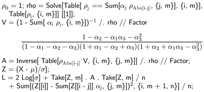
In addition to computing L we have also printed V, as its denominator provides a useful set of if-and-only-if conditions for the process to be stationary (all of its three factors must be positive).

Now, we need to either maximize $\ln LF$ (a difficult task), or make each of its derivatives (with respect to every parameter) equal to zero and solve the corresponding set of normal equations; the latter approach is easier, faster and more accurate; it involves the following steps:

• compute the five ( $2+m$ in general) derivatives of L (the first two lines of the code below); multiply each by σ², thus making them free of σ (with the exception of the σ derivative which, when multiplied by σ³ becomes linear in σ²); denote the results dμ, dσ and dα (the last being a set of m expressions),

Figure 1. Randomly generated data based on AR(3) model.

• similarly (line three), differentiate the extra $\frac{\ln \det \left({\mathbb{V}}^{-1}\right)}{n}$ term of (7) with respect to each α parameter, denoting the answer dV (a collection of m functions of only the α parameters),

• set the initial value of μ to ${\displaystyle {\sum }_{i=1}^n}{X}_i/n$ , of σ (arbitrarily) and of each α to 0, and start the following iteration (performed by Mathematica’s routine ite):

• solve

${d\alpha |}_{\mu }={dV|}_{\alpha }$ (8)

for a new, updated set of α values (the second line of ite; its first line is only preparatory—note its continuation) where ${d\alpha |}_{\mu }$ implies that dα is evaluated using the current value of μ, while ${dV|}_{\alpha }$ is similarly evaluated using the current set of α values; the corresponding equations for the new α’s are thus linear and easy to solve,

• solve

${d\mu |}_{\alpha }=0$ (9)

to get a new value of μ, where the evaluation is now done using the updated α’s (third line of ite); the equation is linear in μ and thus trivial to solve,

• finally, solve

${d\sigma |}_{\mu ,\alpha }=0$ (10)

for σ, where the evaluation is done using the new values of both μ and α (fourth line of ite; the final line just combines the updated values of μ, σ and α’s into a single output); the equation is linear in σ² (its positive root yields the updated σ),

• repeat the iteration till the new values of the five parameters no longer change (a total of five iterations normally suffice to reach an adequate accuracy); this is done by the last line of the subsequent code, which also returns the resulting ML estimates.

To do this, we need to further extend the previous Mathematica code by:

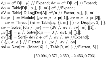
thus obtaining the ML estimates of μ, σ and the three α’s (in that order).

An interesting observation: the last term of L (whose numerator is a sum of squares of differences between predicted and actual values of the Z sequence) always results in 1 when evaluated using the ML estimates returned by sol; this can serve as a verification of the program working correctly.

2.3. Asymptotic Distribution

The general version of central limit theorem (CLT) tells us that the sampling distribution of ML estimators is approximately Normal, with the asymptotic means equal to the parameters’ true values. To get the distribution’s VC matrix, we utilize the theory of Fisher information matrix and

• divide $-\ln LF$ by n, getting

$\ln \sigma +\frac{1}{2}\frac{{\displaystyle {\sum }_{i=1}^n{Z}_i^2}}{n}{\displaystyle \underset{j=0}{\overset{m}{\sum }}}{\alpha }_j^2+{\displaystyle \underset{k=1}{\overset{m}{\sum }}}\frac{{\displaystyle {\sum }_{i=1}^{n-k}{Z}_i{Z}_{i+k}}}{n}{\displaystyle \underset{j=0}{\overset{m-k}{\sum }}}{\alpha }_j{\alpha }_{j+k}$ (11)

where ${\alpha }_0=-1$ ; this follows from (7),

• find the matrix of second derivatives (with respect to each pair of parameters) of this expression,

• find the expected value (indicated by $\mathbb{E}$ ) of each element of this matrix, remembering that

$\mathbb{E}\left(Z_i\right)=0\text{and}\mathbb{E}\left(Z_i{Z}_{i+k}\right)=V{\rho }_k\mathrm{,}$ (12)

• take the corresponding $n\to \infty$ limit,

• invert the resulting matrix,

• and further divide by n.

Leaving out further details, this yields the following results: ML estimators of μ and σ are, asymptotically (i.e. when n is large) independent of each other and of the α estimators, with standard deviation given by

$\frac{\sigma /\sqrt{n}}{1-{\displaystyle {\sum }_{k=1}^m{\alpha }_k}}\text{and}\frac{\sigma }{\sqrt{2n}}$ (13)

respectively, while the α part of the asymptotic VC matrix is

$\begin{array}{l}\frac{1-{\alpha }_1^2}{n}\mathrm{,}\left[\begin{array}{cc}1-{\alpha }_2^2& -{\alpha }_1\left(1-{\alpha }_2\right)\\ -{\alpha }_1\left(1-{\alpha }_2\right)& 1-{\alpha }_2^2\end{array}\right]\mathrm{<mo>\; /\; </mo>}n\text{and}\\ \left[\begin{array}{ccc}1-{\alpha }_3^2& -{\alpha }_1-{\alpha }_2{\alpha }_3& -{\alpha }_2-{\alpha }_1{\alpha }_3\\ -{\alpha }_1-{\alpha }_2{\alpha }_3& 1+{\alpha }_1^2-{\alpha }_2^2-{\alpha }_3^2& -{\alpha }_1-{\alpha }_2{\alpha }_3\\ -{\alpha }_2-{\alpha }_1{\alpha }_3& -{\alpha }_1-{\alpha }_2{\alpha }_3& 1-{\alpha }_3^2\end{array}\right]\mathrm{<mo>\; /\; </mo>}n\end{array}$ (14)

in the case of Markov ( $m=1$ ), Yule ( $m=2$ ) and AR(3) model, respectively. Note that each VC matrix is both symmetric and slant-symmetric (i.e. the same when flipped with respect to either diagonal). They have been found by the first line of the following Mathematica code (by specifying the value of m first).

When executed at the end of the last program (where m was already set to 3), the second line establishes the standard error (using (13) and (14), with parameter estimates replacing their true values) of each of the previously computed ML estimates; note that they are all within two standard errors of their true values.

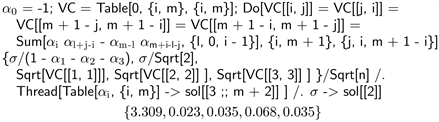
Using these results, we can then compute the standard error of the expected value of the next (yet to happen) observation, established based on (1), the last m observations, and our estimates of μ and the α’s.

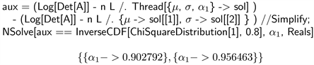
3. Confidence Regions

To construct a confidence region (CR) for true values of all $m+2$ parameters of an AR(m) model, we could directly use their asymptotic Normal distribution of the previous section (see [7] [8] and [9] ). Nevertheless, it is more accurate (in terms of establishing the correct level of confidence), and also notably easier, to utilize the theorem which states that

$2\ln {LF|}_{MLE}-2\ln {LF|}_{\text{true}}$ (15)

has, to a good approximation, the chi-squared distribution with $m+2$ degrees of freedom (notation: ${\chi }_{m+2}^2$ ). Here, the first term of (15) involves the maximum value of $\ln LF$ achieved by the ML estimates, while the second term assumes evaluating the same $\ln LF$ using the true values of the parameters. The proof of a similar statement can be found in [10] ; the necessary modifications are quite simple and need not be elaborated on. The theorem’s accuracy is demonstrated in Figure 2, which compares the empirical histogram of 10⁵ randomly generated values of (15) to the PDF of ${\chi }_3^2$ , using a Markov model with $\mu =10$ , $\sigma =1.7$ , ${\alpha }_1=0.9$ and $n=300$ .

Even though the agreement is not quite perfect (it quickly improves with increasing n), both the accuracy and simplicity of this approach greatly outweigh those of CLT (Figure 6 demonstrates the error of the basic Normal approximation: it is far less accurate than what we see in Figure 1).

Utilizing this asymptotic distribution, we then make (15) equal to a selected critical value of ${\chi }_3^2$ ; solution to this equation yields the CR boundaries. To show how it is done in the case of the above Markov model, we run the program of our original example while changing its first three lines to

This returns a set of data displayed in Figure 3 (the individual observations have been connected) and, after executing the program’s next two segments, also the corresponding three ML estimates (saved in sol).

Computing L and res by the previous routines, and adding the following two lines of code (the first evaluating (15), the second doing the plotting)

produces the desired CR, displayed in Figure 4 (in Mathematica, it can be rotated and observed from any direction).

Figure 2. Empirical and theoretical distribution of (15).

Figure 3. Randomly generated data from Markov model.

Figure 4. 95% confidence region for Markov-model parameters.

3.1. Nuisance Parameters

We have already shown that the three ML estimators of Markov-model parameters are asymptotically independent; this enables us to find a confidence interval (CI) for any one of these (we call it the pivotal parameter) by treating the other two as nuisance parameters (see [11] ). The reference indicates that changing (15) to

$2\ln {LF|}_{MLE}-2\ln {LF|}_{\text{mixed}}$ (16)

where “mixed” implies using ML estimates for the nuisance parameters and the true value of the pivotal one) makes (16) into a ${\chi }_1^2$ type of random variable.

Using parameters of the Markov example of the last section, we display, in Figure 5, the empirical and theoretical PDF of (16), while considering μ and σ to be nuisance parameters and ${\alpha }_1$ the pivotal one; the agreement is nearly perfect.

Let us contrast this result with similar comparison of the actual (empirical) distribution of the ML estimator of ${\alpha }_1$ with its asymptotic (CLT-based) limit (Normal, with the mean of 0.9 and variance, based on (14), of $\left(1-{0.9}^2\right)/300$ ), which is displayed in Figure 6. This time the error of the approximation is clearly inacceptable; using it for constructing CI for the true value of ${\alpha }_1$ is not recommended.

Figure 5. Empirical and asymptotic PDF of (16); nuisance parameters are μ and σ, m = 1.

Figure 6. Empirical distribution of α₁, versus its Normal approximation.

To accurately compute boundaries of a CI for ${\alpha }_1$ , we must thus return to (16) and utilize its fast convergence to ${\chi }_1^2$ distribution. First, we find ML estimates of all parameters (already done in previous section), then add the following two lines of code (the first line evaluating (16), the second one making it equal to the 80% critical value of ${\chi }_1^2$ and solving this equation for ${\alpha }_1$ ):

We then claim, with an 80% confidence, that the true value of ${\alpha }_1$ lies between the resulting two roots.

Note that the theory allows us to designate any set of parameters as pivotal (the rest are then the nuisance parameters); when the two sets of estimators are asymptotically independent, the distribution of (16) is approximately ${\chi }_p^2$ , where p is the number of pivotals. As soon as there is a non-zero correlation between the two groups, the distribution of (16) becomes substantially more complicated and, in the case of AR(m) models, practically impossible to deal with. The technique can thus be applied only to situations when all α parameters are either all pivotal or all nuisance, as demonstrated by our next example.

This time, we generate data from Yule model with $\mu =10$ , $\sigma =2$ , ${\alpha }_1=1.75$ , ${\alpha }_2=-0.9$ , using $n=100$ , by the usual

which produces the sequence of Figure 7.

We then run the common part of the program to find the four ML estimates, saving them under the name res. Executing the following two extra lines (the first line evaluating (16), the second one making it equal to the 95% critical value of ${\chi }_2^2$ , solving for ${\alpha }_1$ and ${\alpha }_2$ , and displaying the resulting contour):

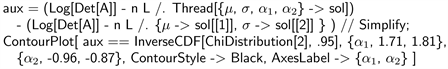
we get the 90% CR of Figure 8 for the true values of ${\alpha }_1$ and ${\alpha }_2$ , while considering μ and σ as nuisance parameters.

This is based on our previous assertion that the distribution of (16) is, in this case, approximately ${\chi }_2^2$ ; to check the accuracy of this statement, we display the empirical version of this distribution (using the same Yule model and 10⁵ sequences of 100 consecutive observations) together with the PDF of ${\chi }_2^2$ in Figure 9; the agreement is again practically perfect.

Figure 7. Randomly generated data from Yule model.

Figure 8. 90% confidence region for α₁ and α₂.

Figure 9. Empirical and theoretical PDF of (16); nuisance parameters are μ and σ, m = 2.

3.2. Establishing Model’s Order

Until now, we always assumed that the value of m (the order of the model) is known; this may normally not be the case, so the question is: how do we test whether an AR(m) model has the correct number of α parameters to be an adequate representation of a given set of consecutive observations? The obvious idea is to see if, by extending the model by an extra ${\alpha }_{m+1}$ parameter, the corresponding increase in the maximum value of the $\ln LF$ function is statistically significant. This can be easily tested by using an extension of the last theorem: when the data does follow an AR(m) model, the following difference

$2\ln {LF|}_m-2\ln {LF|}_{m+1}$ (17)

(where the subscript indicates the number of α parameters used to maximize $\ln LF$ ) has ${\chi }_1^2$ distribution.

We verify this by yet another Monte-Carlo simulation of 10⁵ sequences generated from the AR(3) model of our first example, displaying empirical histogram of the resulting (17) values, together with the PDF of ${\chi }_1^2$ , in Figure 10. The agreement indicates that the latter distribution is again an excellent approximation of the former.

Returning to the original example; we have already computed ML estimates of the five parameters, which are easily converted into the corresponding value of $\ln FL$ . We then need to use the same data and run the same program with $m=4$ , similarly converting the resulting six estimates to a new (always higher) value of $\ln LF$ . Evaluating (17) and substituting the result into the CDF of ${\chi }_1^2$ (we let the reader come up with the corresponding code) yields 0.111; this, being less than 95%, tells us that the data is adequately described by the original AR(3) model.

Figure 10. Empirical and asymptotic PDF of (17); m = 3.

On the other hand, trying to fit a Yule model ( $m=2$ ) to the same data yields substantially higher difference between $\ln {LF|}_2$ and $\ln {LF|}_3$ , resulting (using the same example) in a CDF value indistinguishable from 1 (the corresponding P-value is of the order of 10⁻⁶¹), indicating that no Yule model can properly describe this data.

We mention in passing that, to test the same ${\alpha }_3=0$ hypothesis, we could resort to a less sophisticated approach of using the asymptotic distribution of the ML estimator of ${\alpha }_3$ (Normal, with the mean of 0 and variance equal to $\frac{1}{n}$ , under the null hypothesis), getting a similarly small P-value of 10⁻⁴⁰; this test is not only less accurate (the Normal approximation has a large error, as we have seen) but also less sensitive than the one based on (17).

4. Conclusions

In this article, we have provided a variety of techniques for estimating parameters of an AR(m) model, including construction of confidence intervals/regions and testing various hypotheses regarding parameter values and the model’s order. We have used Monte Carlo simulation extensively to find empirical distributions of various sample statistics and explore the accuracy of each proposed approximation. This led us to conclude that the traditional use of CLT and of the corresponding Normal distribution is to be discouraged due to the resulting large errors. On the other hand, utilizing differences between various $\ln LF$ functions and the corresponding ${\chi }^2$ distribution yielded very accurate results even with relatively small sets of past observations.

There are several directions to pursue in terms of potential future research, e.g.: investigating how flexible AR(m) models are to describe, to a sufficient accuracy, general stationary stochastic processes (such as moving averages) that do not necessarily originate from (1); after all, real data do not exactly follow any mathematical model—these function only as useful approximations. Another possible extension of the current research would be to similarly deal with ARMA models; here, one would need to find some practical way of inverting (and finding determinants) of large symbolic matrices, essential for computing the corresponding $\ln LF$ function.

Conflicts of Interest

The author declares no conflicts of interest regarding the publication of this paper.

References

[1]	Kendall, M.G. and Stuart. A. (1968) The Advanced Theory of Statistics. Vol. 3, 2nd Edition, Hefner Publishing Company, Los Angeles.
[2]	Armour, B. and Morgera, S.D. (1991) An Exact Forward-Backward Maximum Likelihood Parameter Estimation Method. IEEE Transactions on Signal Processing, 39, 1985-1993. https://doi.org/10.1109/78.134431
[3]	Liu, X. and Peng, L. (2019) Asymptotic Theory and Unified Confidence Region for an Autoregressive Model. Journal of Time Series Analysis, 40, 43-65. https://doi.org/10.1111/jtsa.12418
[4]	Vrbik, J. and Vrbik, P. (2013) Informal Introduction to Stochastic Processes with Maple. Springer, New York. https://doi.org/10.1007/978-1-4614-4057-4
[5]	Vrbik, J. (2017) General Formulas for Serial Correlation, Variance and Likelihood Function Relating to AR(k) Models. Advances and Applications in Statistics, 50, 411-421. https://doi.org/10.17654/AS050050411
[6]	Brockwell, P.J. and Davis, R.A. (2002) Introduction to Time Series and Forecasting, 2nd Edition, Springer, New York. https://doi.org/10.1007/b97391
[7]	Phillips, P.C.B. (2014) On Confidence Intervals for Autoregressive Roots and Predictive Regression. Econometrica, 82, 1177-1195. https://doi.org/10.3982/ECTA11094
[8]	Mikusheva, A. (2007) Uniform Inference in Autoregressive Models. Econometrica, 75, 1411-1452. https://doi.org/10.1111/j.1468-0262.2007.00798.x
[9]	Elliott, G. and Stock. J.H. (2001) Confidence Intervals for Autoregressive Coefficients near One. Journal of Econometrics, 103, 155-181. https://doi.org/10.1016/S0304-4076(01)00042-2
[10]	Vrbik, J. (2022) High-Accuracy Confidence Regions for Distribution Parameters. Applied Mathematics, 13, 488-501. https://doi.org/10.4236/am.2022.136031
[11]	Vrbik, J. (2022) Confidence Regions with Nuisance Parameters. Open Journal of Statistics, 12, 658-675. https://doi.org/10.4236/ojs.2022.125039