Can the Capitalist System Protect the Shipping Companies from Business Cycles or They Have to Apply an “Anti-Cyclical” Business Policy? ()
The Capitalist System & the Cycles, the Innovations to Boost People’s Welfare, the Mistakes Committed by Economists about Cycle’s Ups and Downs, Sanko Case-Study
1. Introduction
A shipping company follows a “cyclical” policy when freight rates are high (R1) (Scheme 1). Its ship-owner orders ships—at rather high prices-refraining from scrapping too. When the newly-built ships are delivered (S2)—including the ships ordered by the rest of the ship-owners—they, all together, bring a fall in the freight rate (R2) by increasing supply to S2 (ceteris paribus)!
The “counter cyclical” ship-owner buys and orders vessels—as well as scraps and sells the uneconomic ones—at rock bottom prices—when freight rates are low (R1) (Scheme 2). When he/she receives the newly built ships (S2), freight rates will be high (R2) (ceteris paribus), assuming a rising, but unsatisfied so far, demand (D1 → D2).
The increase of the total supply in the 2nd scheme is lower than the same in the first case (S1S2scheme 1 > S1S2scheme 2) (ceteris paribus). The Perfect Timing, of course, is important (Goulielmos, 2021) , in all shipping transactions, as well
![]()
Scheme 1. The cyclical orders. Source: Author.
![]()
Scheme 2. Counter cyclical orders. Source: Author.
here! This policy is not expected to be followed by the majority of the ship-owners, but only by the “counter cyclical” ones.
The anti-cyclical policy, in other words, pursues the benefits from two worlds: that of the “peaks” and that of the “troughs” of the freight market! Of course, our experience is that the majority of the ship-owners are “cyclical”. This last group is helped by the whole shipping Universe (the banks, the shipbuilders, the scrap markets, the distances probably, the seaborne trade, etc.).
Moreover, the “cyclical” ship-owner believes that the rising of the freight rate (R1 → R2) will stay till he/she shall order new ships, and thereafter, and follows the rule: “the first comes in the market, the first served”. He thus runs to the shipyards so that to participate in the rising profits by obtaining tonnage from the 2nd-hand market soon—and from new-building market—after some time, at rather higher prices…
The novelty of this paper is an exclusive one: “the business cycles for shipping industry—analyzed here clearly as thoroughly as possible—are unpredictable”, and a recommended policy win-win is proposed here. The issue becomes more serious, however, as time goes by: more frequent depressions will appear, where good times will last less than used to be. In fact, we say: ignore shipping business cycles… be prepared our way (epilogue)…stay on top!
2. Paper’s Scope and Organization
The understanding of the mechanics of the maritime cycle—as shown and analyzed here—we considered it, for many reasons, to be the “holy grail” of the shipping industry.
The paper is organized in 7 parts, as follows, after a, rather longer than usual, literature review: Part I dealt with ship-owners and Keynes’ theory of business cycle; Part II dealt with the innovations which societies should prefer; Part III dealt with the way economists understand the business cycle; Part IV dealt with the duration of the freight rates cycles in the shipping dry cargo market (since 1743); Part V dealt with the shipping market cycles between 1945 and 2008; Part VI dealt with the details of the recent shipping cycles every 25 years till nowadays (1997-2022). Part VII dealt with an epilogue. Finally, we concluded.
3. Literature Review
Keynes (1936) explained the BC (pp. 313-332), characterizing it highly complex, as bringing a sudden and a violent crisis (Graph 1)! Keynes born in 1883 and in 1929 depression he was 46 years of age.
As shown, there are 2, important, short-period-variables, which influence the BC: consumption & demand for money. However, the essential character of a BC, its regularity, its sequence and its duration, are due to the fluctuations in the efficiency of capital (Keynes, 1936) ! The crisis comes when the efficiency, (read: its schedule), suddenly collapses (p. 315)! This depends not only on the existing supply of capital goods, and their prices, but also on the current expectation about their future yield, known as “efficiency at the margin2” (Keynes, 1936: p. 317) .
Next, Keynes dealt with how the capital efficiency can be recovered (Graph 2), if it has fallen, and how much time is required.
The recovery of the capital efficiency occurs when the shortage of capital due to its: 1) use, 2) decay and 3) obsolescence, is felt by the economy, (in the case of shipping, the shortage of ships comes from scrapping, and from the ships lost).
Keynes, surely, did not have the ships in his mind, because their average life is long, say about 30 - 33 years, and depends also on the phase of the BC! We have seen ships to “gain” 5 - 6 years extra life in order to enjoy the boom! The reverse, we believe, holds during a depression, where ships will be scrapped 5 - 6 years earlier… out of their average life.
The time now, for the efficiency to increase, depends on the life of the capital. Thus the duration of a slump has a relationship with the life of the durable assets, (and their normal3 rate of growth, meaning the rate at which the newly-built assets are produced, under non-cyclical conditions, we believe).
2Of course this simplicity is based on a rather complex procedure, where the expected efficiency (meaning the net income coming from the future sales of the products/services produced by the capital goods), over capital’s useful life, is discounted to present to be compared with the price to be paid to obtain the capital asset, less its discounted residual value! Here is where the rate of interest enters. The rate of interest cuts-out all investments the efficiency of which is ≤ to the lending cost of money. There are a lot of expected variables to be estimated, the difficulties of which are known to those dealing with the “discounted cost-benefit analysis” concerning present value. Who knows what a freight rate will be 20 years from now? Or, a future IRR-internal rate of return? The BDI index e.g., in end-2008 was 19,000 units and in end-March 2023 was 1456!
3Keynes discussed also the role of depreciation. Depreciation is the saving of the companies out of economy’s income. These amounts are destined to obtain new capital assets. Keynes (1936: p. 104) argued that “consumption—to repeat the obvious—is the sole end and object of all economic activity”.
![]()
Graph 1. Keynes’ Trade cycle is influenced by fluctuations (1936). Source: author. (*) One contemporary question: Can a rising rate of interest cause a crisis? It aggravates & initiates—at times—a BC, but this is not the prime cause (Keynes). Nowadays, we have rising interest rates in the EU, & USA, reaching 4%, to combat inflation… by increasing the cost of money. Better was to increase supply, especially of food products and of energy (gas; oil)! The rising prices do what an increased rate of interest would do, we believe, (they cut consumption)! The reduction in the disposable income due e.g., to dearer home loans, moreover, will bring a recession here in Greece. Those who hold bonds, with fixed rate of interest, are vulnerable, because their market price depends on the interest rate, which lowers their present discounted value (e.g., the “Silicon Valley Bank” case) as it rises. In addition, the rising rate of interest may attract money to the banks, but it may cut-off investments of a lower efficiency than itself.
![]()
Graph 2. The recovery of the efficiency. Source: Author.
4We may remind the reader that the unfinished goods are part of the investment for Keynes.
5Imagine a situation where neither banks nor shareholders are willing to provide liquidity!
As shown, the cost of the unfinished goods4, after a crisis, forces producers to sell them, (a negative investment affecting employment), within a certain rather short period, say within 3 - 5 years, given also that their prices will fall. In shipping this means that the laid-up tonnage will press their ship-owners to scrap them, because their services are not needed anymore in the foreseeable future…
Working capital is expected also to be reduced, as the production will do the same (a further disinvestment). In shipping, we have witnessed difficult situations in which companies found themselves and had to take wrong decisions, because they suffered from a lack of liquidity. A good management has to monitor this and act in advance by having a policy of satisfactory, but not excessive, dividends, as well as a clever depreciation policy, so that to be liquid at all times!
Liquidity is a sensitive issue especially in shipping and it must be secured at all times and at all costs5, as mentioned. The working capital is also essential in shipping meaning the amount of cash required between the time to pay and the time the freight rate is paid, to buy bunkers, pay the insurance premiums, supplies… or repairs.
Efficiency will affect also the propensity to consume, as the market value of the equities will fall (in the Stock Exchanges). A reduction in the rate of interest will have no effect… this time… A far-reaching change in the psychology of the investment markets is required at this stage (Keynes, 1936: p. 320) , but the current volume of investment cannot safely be left in the private hands… Keynes suggests here the intervention of the State.
Keynes replied also to those that considered his BC theory to suggest that over-investment will cause a boom. He agreed only, to that a boom, can be prevented by a high rate of interest! He (p. 320) felt further the need to define over-investment as any “new investment expected to earn—during its life—nothing above its replacement cost!”
A boom needs also a stimulated propensity to consume. Keynes insisted (p. 321) that his typical situation is the one, where, the investment is made under unstable conditions, and destined to disappoint its entrepreneur (a misdirected investment)6. It is very interesting to note that both Keynes and Schumpeter blame the business-men for the cycles!
The Austrian economist Schumpeter (1964: p. 170) (1883-1950)—who wrote an entire book on business cycles (!)—argued in 19397—that “a cycle is designated as a fact, if a given (time) series, displays recurrence of values, (either in its items or in its first or higher time derivatives), more than once” (slightly modified). So, Schumpeter underlined also the characteristic of repetition8 in cycles. We got the impression that Schumpeter—unlike Keynes—talks about cycles lasting between 20 and 30 years!
For Schumpeter (1964) , the entrepreneurs… cause (!) the cycles, as mentioned, as they are the ones playing the leading role in an economy, if they proved especially to be responsible (agents) for bringing-out innovations. But what exactly an innovation means (Graph 3)?
Expansion of the economy occurs, if a number of innovative entrepreneurs exists and acts! The depression adapts economy to the changes which emerged during the boom! This sounds positive for an economy, if innovation reduces the cost of production of a particular product, or of a raw material, as this happened in the treatment of steel in USA!
6In a capitalist economy work business-men, who expect a specific % of efficiency, (>than the interest rate), from a capital good—they could buy—by selling its products during the whole period (life) it will be producing. The expected satisfaction of a business-man’s expectations thus guarantees his/her investment. If now a number of business-men become disappointed, for reasons found in the above description, they will stop investing, and employment will be reduced. Thus, if disappointment is cyclical, investments will be also cyclical, due to a cyclical efficiency too. It is clear that demand/consumption is the one to justify an investment! Apparently, the rising prices will do the same if they boost profits.
7Schumpeter proved to have a wrong timing with his book, because it was published 3 years after Keynes’ General theory, which (GT) challenged all the prior economic knowledge and monopolized the scientific and public interest! Schumpeter, however, did not read “General Theory”, but only the “Treatise on Money”, as he wrote.
8Initially, economists did not deal with cycles… because they considered them as non-re-occurring, like the weather or the earthquakes! This was their first mistake. Thus, the cycles’ repetition/re-appearance was considered essential for economists to deal with business cycles…
Modern economists (Pearce, 1992) defined a BC as the phenomenon which causes fluctuations in the GDP, if it has a regular pattern. It is argued that there is an expansion, followed by a contraction, and a further expansion, while the longer trend is towards up. We ask: Why not towards down?
Stopford (2009: p. 95) adopted Schumpeter’s theory of cycles, we believe. Accordingly, a technological innovation causes a cycle (Graph 4)!
![]()
Graph 3. What an Innovation means. Source: Author.
![]()
Graph 4. The main historical innovations responsible for producing business cycles. Source: Author.
As shown, six innovations were important. The one concerning the fuel to be used by the first motor car, destined, however, to harm the environment by consuming gasoline! So, the entrepreneurs seem to have suffered from myopia, allowing then, and also nowadays, the coal (and lignite) and oil to generate electricity! It took many generations to understand how to produce energy the way Sun does it, even before the Big Bang!
Goulielmos (2017) showed that a shipping cycle—of an average duration of 60 years9—can also be identified (Figures 1-3)!
9Discovered first by Kondratieff’s (1892-1932?).
101) For the Austrian succession, 1740-1748; 2) the American War for independence, 1775-1783; 3) the Napoleonic Wars, 1792-1813 and 4) the American civil war, 1861-1865.
11These are ships with no specific destination acting as taxis of the oceans. Greeks excelled in this type.
As shown, a series of wars10 benefited shipping, between 1741—for which we have data for dry cargoes—and 1871, which is considered (by Stopford, 2009: p. 108 ) as the year-end of the sailing ships. The freight rates increased steadily during this period—till 1813. Thus, a shipping long wave lasted about 80 years (1743-1823); by “deducting” the 21 years of the “Napoleonic Wars” (1792-1813), cycle’s peaceful period was 59 years.
The next shipping long wave started in 1815, and ended in 1870, lasting 55 years!
During the Steam era (1873-1946), the cycles were different (Figure 2). At that time the ships were indeed more beautiful (Picture 1)!
As shown, a Long Wave lasted 73 years between 1873 and 1946. Deducting the 11, or so, years of the 2 WWs, we arrive at 62 peaceful years. This is the period of the so called “tramp shipping11” (1872-1947). The 1918 peak was due to the massive destruction of ships caused by the Great War. It is surprising how this whole period, from 1870 till 1915, and from 1931 to 1947, achieved a freight rate index as stable and as low as round the 100 units (=1870)!
The post 2nd World War Long Wave started in 1947 and ended in end-2008 (61 years). This period is called “bulk era”, due to the appearance of the bulk carriers round the 60,000 dwt and the appearance of the Freedoms replacing the
![]()
Figure 1. The freight rates index for the dry cargo sailing shipping, 1741-1871. Source: Goulielmos (2017) ; a 2-year Moving-Average; used by permission.
![]()
Figure 2. The freight rates index for dry cargo shipping during the Steam era, 1873-1946. Source: Goulielmos (2017) ; used by permission.
![]()
Figure 3. The freight rate market index from 1947 to 2015-the bulk era. Source: Goulielmos (2017) ; a 2-year moving average; index 1947 = 100; used by permission.
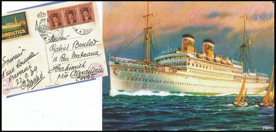
Picture 1. The beauty of a steam ship called “Adriatica”, 1939. Source: Not recorded.
Liberties. It is apparent how the freight market has fluctuated at times (1980; 1995; and par excellence in 2003-2008)!
12According to the theory, the income (GDP/NP) depends on consumption and on investment (and exports less imports, and state’s spending). Consumption, which is the King of all markets, is no doubt influenced by income, but it diminishes as income rises, and is coupled by a rising % in savings. Saving, however, is not a curse, but a blessing, by allowing resources to be devoted to investment—through the banking system. Income obviously, and employment, rise by investment. So, welfare, like a bird, depends on both the wings of consumption and of investment to fly high. Investment, however, is more subjective than consumption, and the bird (the economy) can fly with great difficulty if at all with only one wing! Classical economists wrongly believed that those who save are the same with those they invest, according to the “loanable funds theory”, with moderator the rate of interest.
13This is true as sometimes this information is not disclosed!
14Under normal (non-cyclical) circumstances this is not so, and should not be so!
Summarizing, it is clear that from Science’s point of view, there is… a family of business cycles! From the side of businesses, it is also clear that cycles start and end by the business-men (“mea culpa”)! The business-men form certain long-term expectations concerning their markets, but markets obey the supply and the demand, and, from time to time, they disappoint them. Here is when a cycle starts… The disappointed business-men withdraw12 from ordering capital goods, and a slump begins! When the market verifies the long term expectations of the business-men, they then only start to order capital goods, and recovery begins.
4. Part I: Ship-Owners and Keynes’ Theory of the BC
Ship-owners, in order to build ships, consider first “what net profit is expected to be derived from them till scrapped”. Their expectations are based on a very precarious basis, which is subject to unreliable and shifting evidence, and to sudden and violent changes! This is true, if one takes into account the many global and local wars and the 2 canal closures, which have already occurred and disrupted the normal evolution of most of the world economies!
Ship-owners pay attention primarily on the current freight rate, and they do not care too much about what others are building13, or they are not deterrent by what the current newly-built-ship price is14! What, however, is substantially true, is that they are unable to know what the ship’s future yield is going to be. Moreover, in a lesser degree than that assumed by Keynes, we believe, ship-owners care about the rate of interest15 and their cost of finance!
The above behavior—in a case of rising freight rates—shall increase the supply of newly-built ships, reduce the freight rates, and collapse their efficiency, as shown by the graphics in the introduction! Keynes gave particular emphasis on the uncontrollable psychology of the business-men (p. 317), as the main characteristic of capitalism. The return of confidence to the market is required… after any disappointment! This means that when the expectations of the business-men, about efficiency—are verified by the market, confidence returns!
Our research experience taught us that scrapping—on which a ship-owner may place his/her hopes for a fast remedy of a crisis—is a very slow procedure, taking up to 3 years to correct an oversupply, depending also on its volume! Scrapping, and its time, we consider them as the main responsible factors for a depression to depart. But, the rather faster reaction of ship-owners is not to scrap, but to lay—unprofitable ships—up, within say 3, or so, months, since the freight rates fell permanently! The laid-up tonnage is a temporary action for a lower supply. This, rather clever, shipping mechanism—i.e., of the lay-up—appears when the ships become “sick” (bringing losses) and go to their “hospital”—(the anchorage)—till their health is restored (the market improves). If the market delays to improve, (meaning that the therapy is going to be delayed), the patient will die (scrapping).
Ships have a long average life of 30 - 33 years, or so, which, however, even this varies in accordance with the state of the market, as mentioned! This influences the shipping cycle! The further extension of the life of the ships, obviously maintains the status quo, which is expected to change only by the delivery of the newly-built ships and scrapping (or loss) of the others! This further proves that the shipping cycle’s time is changeable.
We identified the “stock of the unfinished goods” (Keynes)… with the “laid-up services” of ships! The laid-up ships exert a pressure on their owners to get rid of them, because they bring further losses to them—i.e., cost to place them in an anchorage, and stay there, and cost to prepare them to carry cargoes again.
15Given the substantial amounts that have to be devoted for building e.g., an LNG carrier, at a price of $200 - 250 m… and the interest to be paid on a 80% loan.
Important role plays also the ships’ scrap value, which became higher when ships became larger (due also to the scrap price, which in a boom is high). This change brings a faster equilibrium between supply and demand. The volume of the ships in the anchorages prolongs the length of the shipping cycle by preventing supply to fall!
Therefore, the shipping cycle is a complex phenomenon, where many factors work in a positive way and others in a negative one, as follows (Table 1).
Any gap between demand and supply (when D > S) of ship space for hiring, needs time to be absorbed. Surely, if the “ship-building time” increases—here assumed 2 years—the boom will be prolonged (given distances). Also, the crisis
![]()
Table 1. Positive & negative influences working towards a shipping cycle.
Source: author.
will be prolonged, if the laid-up decision takes a longer time than the 3 months assumed here; the crisis will be, however, shortened, if the scrap decision is taken earlier than in the 3-usual-years assumed here. Certainly we saw few cases of cycles to last about 11 years (1958-1969) and about 9 years (2009-18).
4.1. The Technological Progress in Ships
Shipping, no doubt, is a par excellence sector—together with shipbuilding—where applied technological progress is embodied (Graph 5) (Goulielmos et al., 2021) . The internal combustion engine e.g., though used oil, was important for all users then, and now. Nowadays, the car-manufacturers, using such engines, are called to stop it, facing the strong opposition of Germany, and of France, which wishes to produce hydrogen using nuclear power.
As shown, technology helped ships to become faster, larger and having a reduced crew, especially by automating the engine room during the night (Japan); also, to use cheaper fuel and to install economy main engines—after the 1st and 2nd oil crisis (1975; 1979).
16This makes transport cost lower. Any cargo has a value and thus embodies funds which pay interest. The interest period shortens if the transport time shortens. This is more important when the unit value of the cargo is high! This is why very valuable cargoes prefer the air transport or the liner shipping.
Additionally, stronger gears, reliable hatch-covers, larger openings in driving cargo into the holds; better radars and improved navigation via proper routing; better telecommunications, and a satellite, etc. Moreover, we had more effective, if not, more efficient, ports. Fleet’s productivity improved16 by leaps and bounds…
What is left? The ships to become digital-smart, applying AI, burning a friendly fuel to the environment! Of course, we have to ask, if all the above remarkable achievements made with the help of technology, will reduce the cost of sea transport in their CIF expression? Stopford (2009) argued for the past that they did. This, however, is worth of further research for our future.
![]()
Graph 5. The main Innovations in the shipping industry. Source: Author.
4.2. Can the Capitalist Economic System Provide Protection to the Companies from a Coming Business Cycle?
Theoretically, we know that the best economic system is the one which eliminates monopoly profits (Figure MN1)! This system, however, is defective because it does not give a specific time for this to be accomplished! And the elimination is unfortunately done after the monopoly profits have been obtained!
As shown, Perfect competition determines a freight rate equal to 0F2, where AC = demand. A Monopoly market determines freight rate at 0F1, where MC = MR, given demand. Monopoly reduces production (from 0M to 0L), but this is not true for shipping. In shipping, OF1 is paid for 0M tonnage dwt, as in 2003-2008. Here, we do not mean that thousand of shipping companies become suddenly one, as theory implies, but each enjoys 0F1 at different average cost each. 0F1 is determined by Supply and Demand, where D > S.
5. Part II: The Innovations Which Societies Should Prefer
We talked above about innovations. In our opinion, we have to add here, the benefits from a proper way of creating innovations, which comes from applied research, from the universities, or from dedicated applied research centers. It only matters, personally—if innovations focus on and achieve-out—a better quality of life! Great nations are characterized by the amounts devoted to applied research, but not also by the degree of reinforcing their welfare state, as they should…!
It is apparent that we need a criterion to connect innovation to the “welfare” of people, which we consider it to be the most important task! Let us call them “Welfare Innovations”-WI. Modern economists failed to define innovations in our way, and restricted the whole issue in production. We will define a “welfare-producing innovation”-WPI then: “This is the one which contributes
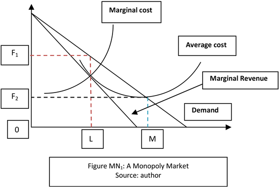
Figure MN1. A monopoly market. Source: Author.
towards establishing a ‘welfare state’ and/or promoting the existing ‘social welfare state’ in a rather continuous pattern!”
We are aware that 80 years have already passed from the famous “Beveridge Report” in UK (1942), conveying similar ideas as ours. This must be revisited. We believe that this activity—of increasing people’s welfare—should be organized better than hitherto, and to incorporate also the private sector. A ministry, called “People’s Welfare”, also, to administer properly the hundred benevolent houses and foundations in a country (and in Greece) for a coordinated action and better results to the benefit of the people in need, using the digital technology!
We will give an example for what we mean when we say an “innovation to boost the welfare state”. This is what has been called the “Holy Grail” of the energy production, a method producing energy by imitating the Sun (Graph 6).
As shown, this important innovation, which consumes less energy to produce more energy, may contribute to diminish the cost of energy to households, increasing thus their welfare! It is well known that the higher the prices, the lower the quantities of consumption, and the lower the level of welfare! The lower the prices, the more quantities a fixed income can buy, thus increasing welfare! We talk here only about body’s welfare—as this is the sole interest of economics—but we can work-out and the welfare of the soul!
Thus our definition focuses on those innovations which increase society’s welfare, and not only the profits of the companies, if these profits are distributed only to their shareholders, without a portion of them to go to their community. A 2nd example we could mention is the by-products of the NASA research, if those again come-down to people’s welfare.
Before closing this part, we will mention the international effort to establish a mandatory reporting about: 1) a company’s impact on environment; 2) its social policy for its employees and its community, and 3) its governance (ESG)!
![]()
Graph 6. The nuclear Fusion, 2022 (“US National Ignition facility”). Source: author; information from the internet.
In our opinion, ESG has to be broadened to concern all, and not only companies, as hitherto. When we say all, we mean especially those who: 1) can reduce their carbon emissions; 2) contribute towards a better climate; 3) diminish their general pollution; 4) reduce their waste disposals; 5) pursue renewable energy sources and 6) prevent the resources’ depletion or work for their increase. The above to have a tax reduction or other rewards, and get an ESG decoration!
The ESG must concern all energy users, in particular, and naturally the Ships! Moreover, long-term research is urgently required to be completed for the role of the quality of the environment on the “creation” e.g., of certain deceases, including cancers! If a correlation is found strong, as recent evidence shows, then we will know why the health budgets increased, and why all schemes of social health failed… The quality of life has inevitably been greatly reduced over the years! Societies must care to have fewer sick people, by educating people in the schools about what factors, and why, shorten their life!
Instead of creating more and more medicines, presumably for any and all deceases, existing, or coming, is better to prevent them, using the existing natural ways. We have to teach people to follow the “hygienic way of life” and free it from stress, smoking, accidents and drugs to start with. Life is valuable and has not to be wasted as it only gives the opportunity to love one’s neighbor!
6. Part III: The Way Economists Design the BC
The business cycle—as drafted by an economist in 1992-was as follows (Figure 4).
As shown, a trade cycle has 2 peaks: B and F, and 1 trough: D. The cycle starts at A, (or B), and ends at E, (or F). It has 1 symmetrical hill and 1 valley also symmetrical. Cycle’s amplitude is equal to BG. The contraction is equal to BCD, and the expansion is equal to DEF.
Worth noting is that the above cycle is unusual, because DEF = BCD! This is an obvious mistake! This is also contra to the popular wisdom arguing that the “good times are shorter than the bad ones”… In the real business life DEF < BCD,
meaning that the “expansion” is almost always shorter than the “contraction”! There is one exception, however, that of the 2003-2008 exceptional boom!
When we come to maritime economists, surprisingly, the same mistake, as above, is committed! Stopford (2009: p. 102) , assumed an almost symmetrical shipping freight rate cycle (Figure 5), where a peak A is almost equivalent, or close, to a trough B, given time!
As shown, a shipping cycle has a peak almost equal to a trough: A ≈ B. This, however, does not correspond to reality, where depressions last always longer than booms (A < B), except in a situation of an exceptional boom as mentioned!
Figure 6, indicates that the contraction and the expansion periods, and thus shipping cycle’s entire period, as well cycle’s amplitude, not only vary over time, but also the peaks—taken together—are longer than the troughs, or A > B in this particular period of the exceptional boom!
As shown, all indices of the freight rates—for 3 dry cargo types and 1 general—between 2002 Jan. and 2008 (Oct.), showed a 8000 units amplitude in 2004 (in Capes); 9000 in 2005; 16,000 in 2008-1st quarter—and 19,000 in 2008-3rd quarter!
Moreover, 1 short cycle lasted 12 months (2003-4); the 2nd very short cycle lasted 7 months & 15 days (2004-2005); there was a long trough till 2007 (2005-2007; of 25 months & 15 days) and 1 final cycle lasted from 2007 to 2008 (13 months & 15 days) (total 58 months and 15 days or almost 5 years)! The trough covered about 18% of cycle’s time and the peaks 82%. This is so, for otherwise it would not be recognized as an exceptional boom!
Thus, the above data proves that 4 short peaks can emerge, lasting 33 months, and also 1 long trough lasting 25 months and 15 days! This, not only destroys the idea of equality, in time, between ups and downs of the freight rates, but also proves the fact that one rather frequent shipping cycle lasting 5 years (2003-2008), (this happened also in 1981-1987 = 6 years), can accommodate 3 shorter cycles! This boom conveyed also another message, which is that the monopoly profits led to excessive orders of ships thereafter and as a result to a longer depression (of 10 years)!
So, there is indeed an issue here of how long a shipping depression can be and how long a shipping boom can be? We turn now to this specific issue.
![]()
Figure 6. The 4 shipping freight rates indices in quarters, 2002 (Jan.)-2008 (Oct.). Source: Baltic.
7. Part IV: The Duration of the Freight Rates Cycles in the Shipping Dry Cargo Market, since 1743
Stopford (2009) devoted a whole chapter to shipping cycles (pp. 93-134), quoting a ship-owner to say: “When I wake-up in the morning, and the freight rates are high, I feel good… and when are low, I feel bad” (1995). This quotation indicates that the ship-owners’ feelings are determined by the level of the freight rates!
7.1. The 1743-2003 Period
Using Stopford’s data, since 1743, we plotted the peaks and the troughs of the dry cargo shipping freight rates index over 266 years17 (Figure 7), by indicating their duration in years.
As shown, the duration of the troughs, (red columns), lasted longer than the duration of the peaks (blue columns). The data has interrupted by 3 wars (Numbers 5, 13, 16: Napoleonic, Great War & 2nd WW). Since 1947 and till 2008, 8 peaks were shorter than the respective troughs, except in 1979 (number 22) and in 1988 (number 23), explained below.
17 Stopford (2009) explains analytically the sources of his data, since 1741, p. 104-107. He found 22-24 cycles lasting 10.4 years on average (1743-2007).
So, if we want to be honest with our ship-owners, we have to tell them that a depression will last longer than a boom as time goes-by! During the last era, 1947-2007, called “bulk”, the market produced 8 peaks—of an average duration of 3 years—and 7 troughs—of an average duration of 5 years (total 8 years).
The above, finally, proves that the good years covered 37.5% of the cycles and the bad years 62.5% of them. Thus ship-owners have to be prepared to face this
![]()
Figure 7. The duration of troughs & peaks in dry cargo shipping freight rates index between 1743 & 2003 (in years)—24 various not continuous years. Source: data from Stopford (2009) .
reality, probably time-chartering their ships when they are found themselves in the 37.5% situation! The 2003-2008 exceptional boom is, however, a marked exception!
Worth for further research is the fact that since 1743 to 2008, both peaks and troughs diminished in duration, as follows: during the sail era the average peak was 6.1 years; in tramp era, 2.6 and in the bulk era, 3. The average trough was 8.7 years, 6.7 years and 5 years respectively (Stopford, 2009: p. 106) . The phenomenon, of the shortened booms etc., is worth researching further so that to pre-know what we have to expect in future! We may ask for the time being: is the above pattern, of shorter and more frequent cycles, due to the higher average speed, which ships obtained? Or is this due to the economies of scale that ships embodied? Or is this due to the lesser time spent in ports by the ships? We believe all these count.
Stopford (2009) attributed the above phenomenon—of the shortened booms—to technology, and/or to global communications, which emerged since 1865 (p. 107). What about our era where the “smart phone” is the essential companion to all persons? No doubt the more rapid communications may speed-up production, and may solve problems faster by intensifying control—so important for shipping!
The above developments surely mean that demand is served faster than used to be, meaning that the technology made… the depressions to arrive sooner and to be more frequent! Also, the peaks made shorter, and lasting less, contra to what Schumpeter (1964) and Stopford (2009) argued in praising the benefits derived from the innovations!
18This policy of copying other ship-owners in their investment strategy followed also by Greeks. Greeks, when they saw large successful shipping companies to order ships they thought that it is proper for them to do the same, because the large companies should know better something the smaller ones did not! Of course this is a dangerous policy because even the big companies commit mistakes!
Economists, however, cannot explain the above paradoxes involving time, because, to start with, time—as a variable—has been absent from economic analysis (Goulielmos, 2018) . We leave this issue for further research. In shipping, time is an essential element, as the faster production allows for a higher income, at the unit of time—let it be one year! This is why ship-owners asked for higher speeds and larger vessels and less loading/unloading times in a port during a boom! They know better!
7.2. The Wrong Assumptions Made-Out by the Sanko Shipping Co of Japan—A Case Study
In 1983-1984, freight rates for bulk carriers were depressed, but surprisingly, certain companies placed orders! A Japanese company, named “Sanko”, placed orders secretly by ordering 120 ships (about 30,000 dwt each)—but it has been followed by the Greeks and the Norwegians18! This movement was considered as a “counter-cyclical” (Stopford, 2009: p. 126) from the side of the Japanese company!
A number of preconditions were indeed favorable to trap any shipping company at that time, not only Sanko, because: 1) The 1980 boom supplied companies with enough cash; this further means that the behavior of the ship-owners is different if they come-out from a depression, or if they come-out from a boom, as mentioned; 2) banks wanted to lend-out their petrol-dollars; 3) ships were cheap—shipyards were full—and orders for tankers were zero, due to their crisis in 1975 and in 1979; 4) Shipyards were offering a new generation of “fuel-efficient bulk carrier” given the very high oil prices, after 1975 and 1979 oil crises; 5) the Yen to $ parity was favorable.
Moreover, and most important for this work, is that the owners (Sanko), by ordering in 1983, they were expecting a cycle lasting 2 × 2 = 4 or 5 years—as the previous one (1975-1978 down; 1980-1 up), and thus the delivery of their ships planned for 1985—would be at rising freight rates! It is important to stress here that the Japanese expected the delivery of ships to coincide with the upswing of a cycle spending 21/2 years-up and 21/2 years-down!
This case-study delivered also a 2nd important lesson: the supply of ships is not unaffected by the supply of even 1 shipping company—as assumed by Perfect competition, given its volume. In this case-study, it is estimated that the 3.6 m dwt ordered only by “Sanko”19 were able to depress a low market even further! This indeed caused the freight rate index to fall from 300 units to 50, and the recover to delay 11/2 years—till 1987!
8. Part V: The Shipping Market Cycles (1945-2008)
This period produced… 23 peaks, till 2008. We will remind, however, the facts that caused them (Table 2)!
19Sanko had a strong political support, dealing first exclusively with tankers, and having accessibility to the banks. This tanker exclusivity was company’s 1st mistake. Given that tankers delivered losses, Japanese thought it proper to enter into the bulk carriers, by creating such a fleet, which would make a profit equal to the tanker loss (a right thought)! But they could have been finally right, however, if they assumed that the shipping cycle might last 6 years (1981-1987) as it did, and the depression 4.5 years (1981-1985), as it did, and the orders to have been placed in 1985, instead of 1983!
As shown, this period, of 63 years, had everything: local wars: in Korea; Iran/Iraq; Iraq/Kuwait; Iraq with USA coalition etc.; 2 closures of the Suez Canal, 1956 and 1967; 2 oil crises in 1975 and 1979; one revolution, in 1979; one shipping depression, in 1981 and one exceptional boom (2003-2008)! All the above events were impossible for any ship-owner to foresee…
The essential impact, however, created by the 1st Suez Canal closure in 1956. Ship-owners, including Onassis, believed that the Canal will be closed for a long time, and as a result they run to shipyards to build super-tankers, which would be able to make the longer journey round Africa (Cape of Good Hope—Map 1)!
But the Canal re-opened in 6 months, and the oversupply collapsed the freight rate market! This is a mistake committed by the ship-owners, and no shipping cycle can be held responsible! The “1979-1987 cycle in tankers” had also as a result for tankers to stop influencing the dry cargo ship market. Moreover, the crises in tankers, in 1975 and in 1979, in a way, warned the dry-cargo ship-owners of what was coming, and they were prepared in 1981 (2nd half)! Moreover, the
![]()
Table 2. Bulk shipping market cycles, 1945-2008.
Source: data from Stopford (2009: p. 118) .
![]()
Map 1. The cape of the good hope. Source: Internet.
nations with extended tanker fleets paid a higher toll-like Norway, and unlike Greece (Goulielmos, 2023) .
The Period: After 2008
Of course, between 2009 and 2022, we had 1 additional local war, which really is the 3rd global one, (Ukraine & NATO against Russia) (2022 Feb.); 1 global financial crisis (2009-18) and 1 Pandemic (2019-2022)! Inflation (2022-).
Worth noting is that the local wars, the pandemic, the famines, the earthquakes, the fires, the floods, the droughts, the high temperatures, etc., are expected to continue to emerge and is better for all nations to be prepared! For Peace perhaps something else stronger is required…from all nations!
9. Part VI: The Shipping Cycles since 1945 in Detail
9.1. The Cycles between 1945 and 1969
Shipping faced high demands given the enormous needs, which the 2nd WW created, and the scarcity of tonnage—due also to Wars. The freight rates obtained soon a high level, where the golden combination prevailed: “high demand, low supply” (for sea transport). This led ship-owners to their classical reaction to order ships. The market started to fall (1947) and to reach a low point (1949), and to become calm (1950). This cycle was a combined product mainly of demand, & Supply.
The demand exploded (end-1950), because of the Korean War, which caused a stock-building panic, and a raising seaborne trade (16% in one year—1951)! Demand, next fell, because the war finished (spring 1952), freight rates fell (by 70%), the laid-up tonnage increased (1953). The 2nd hand ship prices fell from 1/2m pounds, (end-1951), to £230,000, one year later (for a liberty b. in 1944)!
The market started to improve (2nd-half of 1954), and by year’s end, freight rates increased (by 30%), and continued to improve (1955-1956), when Suez Canal closed! This was the big unexpected event of this period, as mentioned, and as a result it produced 2 cycles (1956). So, cycles can be triggered by unexpected serious events like the closure of a vital canal, or by a war!
The next year (1957) produced rock-bottom freight rates (index = 50 units; 1947 = 100), and led to a 10-year depression—till and beyond 1967-when Suez Canal closed for the 2nd and more lasting time! The canal’s closure increased demand by increasing distances! Certain companies signed contracts for tankers… that had to be built. The eventual reopening of the Suez Canal reduced the existing demand…
In fact, we cannot blame this time the seaborne trade for the above cycle, which rose from 990 m tons to 1790 m (1959-1966 or 80% in 7 years). This cycle is obviously due to oversupply and the ship-owners were clearly responsible…
Table 3 indicates the additional factors, which played a role in this long cycle (1956-1969) of 14 years in the dry cargo sector!
![]()
Table 3. The reasons for the decline in dry-cargo markets, 1956-1969.
Source: data from Stopford (2009: pp. 121-123) .
9.2. Cycles from 1970 to 1987
This period created 3 bulk carriers’ cycles. The responsibility for this, this time rests on seaborne trade, which was the real cause of a buoyant market (it increased by 78%, from 1966 to 1973, from 1807 million tons to 3233). Shipbuilding was unable to respond. Moreover, the 1971 recession was short.
Great prosperity and expansion occurred in shipping (1970-2)! The freight rates of ore-carriers improved. The “Tap pipeline” closed (May, 1970). Libyan production of oil restricted, and moreover its nationalization (1973, August) took place; distances rose. The 1973 was exceptional! A VLCC, earning $22,000 per day in winter, earned $44,000 in summer.
The tanker market, however, collapsed after the “Yom Kippur war” (1973). The dry cargo market resisted somehow (1974-1975), depending on ships’ size. The good times were due: 1) to the buoyant economic growth; 2) the stock building due to inflation and 3) the heavy congestion in the M East and Nigerian ports (1975).
Then, tankers met their disaster (1979-1987), following their prior stage of over-building (1970-1980)! Responsible this time was the oil price (the OPEC)! It rose from $11 per barrel to about $40, due to the revolution in Iran (1979), reducing20 oil seaborne trade (from 1.4 b tons to 900 m in 1983)! One out of 2 tankers was redundant by 1981-83 at W = 17 - 20 units!
Scrapping was the only solution for the 40 m dwt (1982) and 53 m (1983) in anchorages. This depression (-1985) was considered equivalent with that in 1929-1933! In 1986 signs of improvement were shown, triggering heavy investments in new tankers including speculative ones…
9.3. Cycles between 1988 and 2008
After the tanker markets reached their bottom (1985), and the dry cargo ones their own, a year later (1986), conditions started to improve by 1989. In 1990, the destiny of tankers turned to be different from that of bulk carriers (-1995) by having different investors, as mentioned.
20This tanker depression (1979) could be more severe, if economies did not use coal on received lessons since end-1973 to seek for alternative sources of energy away from oil! This is unlike the 2022 gas and electricity crisis due to the Russia-Ukraine war, which caught EU sleeping… As result the last depression 2022-2032 will be indeed really long…
21In shipping standards do not exist. Here tankers assumed to live 20 years! But they did not.
22A new VLCC in 1986 priced at <$40 m and in 1990 priced over $90. In 1995 the shipbuilding capacity more than doubled from 15 m dwt to 33 m.
23Oil sources from shorter distances emerged!
The tanker ship-owners took—at last—their revenge by embarking on heavy orders amounting at 55 m dwt (1988-1991). This made out on 3 main expectations: 1) the fleet, of ageing tankers—built in 1970-1980—expected to be scrapped (during 1990-2000), and replaced21 (1995); 2) the shipbuilding capacity fell (1980-1990), something verified also by the rapidly increasing shipbuilding prices22; and 3) a growing oil demand expected from the Middle East23, favoring the VLCCs, due also to longer distances. But none of the above expectations of ship-owners verified! As a result, a shipping BC (1992-1995: a 31/2 years recession) created by the unfulfilled expectations. Keynes was right!
The non-tanker owners now ordered less than 1/2 of that of their tanker colleagues (24 m dwt) (1988-91), and they were receiving 4 m dwt p.a. (1992) (1/4 of that of tankers), peaking-up soon (1995). But the bulk carriers by having earned during 8 years enough profits (1988-93) (1993-95), managed to order 55 m dwt as tankers did before! The deliveries (1996), and the Asian crisis (mid-1997), triggered the new BC24 (Stopford, 2009: p. 129) .
In the spring 2000, the situation changed. As argued by Stopford (2009: p. 129) “as so often happens in shipping cycles, things did not develop as anticipated, and the market experienced a classic boom-and-bust-cycle (1999-2001)” (bolds added). A boom25 occurred then after 25 years! The 2001 collapse of the internet stocks, unfortunately, triggered the next depression. A VLCC earned only $10,000/day and a Cape $6000. The exceptional boom had, however, to come later (2003). Responsible for this was…China; its infrastructure developed by importing from 144 m tons iron-ore to 468 m (2007), plus imports of oil.
24A tanker earned $37,000/day in mid-1997; and <10,000 in Sept. 1999.
25A VLCC earned $80,000/day in Dec. 2000.
26Members will be definitely China and India.
The above stories led us to propose the formation of a group of the 10 big26 global “exporters and importers”—let name it the “G-10-big sea traders”, to agree as to what sea exports and imports each country has to undertake for the global rate of growth to be secured! The nations, nowadays, must undertake not only their national obligations, but also their international ones, given that the world is a common village! Due, however, to Ukraine-Russia war, the villages now came to be three: Russia and its allies (Belarus, Hungary etc.), NATO and the Neutrals (China).
10. Part VII: An Epilogue
The above destined to show that in order to manage a BC—we have to anticipate also a great and frequent number of non-economic factors, especially the local or global wars…
Stopford (2009: p. 130) struggled—rather hopelessly—to adopt a definite duration for the shipping business cycle. He first brought coal to Newcastle by saying that the shipping cycles exist! Then, he provided a statistical average of the shipping cycle of 7 years, but this was not supported by reality; the last 50 years showed cycles of 8 years on average!
The weighted average cycle calculated by us gave a cycle time near 6 years for 12 cycles during the last period! Stopford then argued that if he was a bank manager, he would not believe in a 7 years cycle, if the money in a company finished in 9 years! The recent 2003 boom gave a cycle of 5 years! The GFC gave a cycle of 10 years.
Our suggestion to our friends, the ship-owners, is to forget the uncontrollable shipping cycles, and to buy/build ships at rock bottom prices, larger and younger than those owned hitherto, and perhaps sold; to sell then their older and smaller ships. The 2nd hand may be of 5 years of age a providing many advantages.
The above recommended anti—cyclical policy will secure benefits from the economies of scale and from the economies of age. Attention is drawn to the fact that this policy, in order to be fully successful, must be done at real rock-bottom prices…and not at prices believed to be such. Greek ship-owners by doing our suggestions reached in March 2023 to own 349 m dwt (Figure E1)!
As shown, the years 2008-2013 expressed the impact from the 2009-starting depression, where the fleet then regressed from 261 m dwt to 265 m. This repeated in years 2018-2023, where the fleet regressed from 342 m dwt to 349 m. These two periods further reveal a 2 × 6 years depression!
During the exceptional boom, 2003-2008, the fleet added 89 m dwt (within 6 years)! Our experience has taught us that no fleet is un-vulnerable to global crises, more or less. The next year—2024—is expected the Greek-owned fleet to add 15.4 m dwt, now on order, and to reach ~365 m (ceteris paribus: scrapping and losses in marine accidents and sales/purchases to/from non-Greeks).
11. Paper’s Limitations
The paper could be more convincing, if the detailed predictions about every separate freight market made in the past, brought-up and showed-out why they failed. This paper assumed the widespread opinion that freight rate markets are un-predictable, even among scientists! The paper, however, indicated the way—perhaps in fewer words than deserved—of how to get rid of the unpredictability! The cycle matters if one cannot buy and build ships at rock bottom prices—ships bigger and younger. Also, if one cannot sell ships smaller and older. In our opinion every clever ship owner can do this if prepared and disciplined.
![]()
Figure E1. Greek-owned shipping, 1988-2023 (March) dwt.
12. Conclusion
The capitalist economic system cannot prevent a business cycle! Moreover, the “boom profits” exerted a pressure on ship-owners to order ships (in 2009 and thereafter). The boom profits prolonged the shipping depression (2009-2018), making the situation worse. The last time, BC has been caused by the Global Financial Crisis (2009-2018) was due to the decease of the capitalist banking system: the greed.
Many prominent general economists, including Keynes, and fewer maritime ones, including Stopford, wrote about the so-called “trade cycle”, known nowadays as “business cycle”-BC. This was very popular subject in the past, till growth economists, in 1940-1950, dropped it out of the agenda. For ship-owners, however, this is, and was, a frequent issue, which they could not fully understand, let alone manage. Maritime economists are also confused!
The economic theory provided many versions to describe a rather complex problem—as that of the BC—and people have been, and still are, also confused as to what causes a BC, and how it can be avoided. If all economists, writing about the BC, are right, then we must have as many causes, for the BC, as there are writers! One thing is certain: the BC plays with time!
The BC has to be studied in accordance with its time length, if one wants to get down to meaningful conclusions, we believe! Economists did this by instinct, and made a taxonomy of cycles combining 1 name and 1 duration, like: the “Juglar” cycle, meaning the 10-year one; the “Kitchin” cycle, meaning the 40 months one; the “Kondratieff” cycle, meaning the 60 years one; the “Kuznets” cycle, meaning the 25 years one; the “Keynes” cycle, meaning the 5 years one; the “Schumpeter” cycle, meaning the 30 years one…
Moreover, it would be more fruitful not to consider one scholar wrong, because he/she argued that the cycle lasts so many years, and another right, because he/she believes that a cycle lasts a different amount of years. As shown, all cycle durations are candidates!
We believe that the existence of fluctuations of different span and intensity are worth searching. Greek ship-owners, however, made Keynes’ theory invalid by getting no disappointment from their capital investments, as mentioned in the epilogue!
The capitalist system indeed can only work towards restoring the cycle’s abnormalities—after the event—by consuming certain time, varying in accordance with the seriousness of the situation, and the gap between demand and supply! Companies, however, have to rely on their counter-cyclical strategy, as Greek ship-owners do. This is the important conclusion of this paper.
We were surprised, however, as to how the long waves demonstrated by Kondratieff for the main capitalist economies in the 1920s, can be manifested also in shipping! This tells us further that shipping is sensitive to global economic situations and the wars… for the last 282 years!