The Bivariate Normal Integral via Owen’s T Function as a Modified Euler’s Arctangent Series

Janez Komelj

Independent Researcher, Vnanje Gorice, Slovenia.

DOI: 10.4236/ajcm.2023.134026                

Abstract

The Owen’s T function is presented in four new ways, one of them as a series similar to the Euler’s arctangent series divided by 2π, which is its majorant series. All possibilities enable numerically stable and fast convergent computation of the bivariate normal integral with simple recursion. When tested  computation on a random sample of one million parameter triplets with uniformly distributed components and using double precision arithmetic, the maximum absolute error was 3.45 × 10^-16. In additional testing, focusing on cases with correlation coefficients close to one in absolute value, when the computation may be very sensitive to small rounding errors, the accuracy was retained. In rare potentially critical cases, a simple adjustment to the computation procedure was performed—one potentially critical computation was replaced with two equivalent non-critical ones. All new series are suitable for vector and high-precision computation, assuming they are supplemented with appropriate efficient and accurate computation of the arctangent and standard normal cumulative distribution functions. They are implemented by the R package Phi2rho, available on CRAN. Its functions allow vector arguments and are ready to work with the Rmpfr package, which enables the use of arbitrary precision instead of double precision numbers. A special test with up to 1024-bit precision computation is also presented.

Keywords

Owen’s T Function, Bivariate Normal Integral, Euler’s Arctangent Series, Recursion, R Package Phi2rho

1. Introduction

Let $\Phi \left(x\right)=\frac{1}{\sqrt{2\pi }}{\displaystyle {\int }_{-\infty }^x}{\text{e}}^{-\frac{1}{2}{t}^2}\text{d}t$ be the standard normal cumulative distribution function (cdf) and $\phi \left(x\right)=\frac{1}{\sqrt{2\pi }}{\text{e}}^{-\frac{1}{2}{x}^2}$ the standard normal probability density function (pdf). The bivariate standard normal cdf

${\Phi }_{\rho }^2\left(x\mathrm{,}y\right)=\frac{1}{2\pi \sqrt{1-{\rho }^2}}{\displaystyle {\int }_{-\infty }^x}{\displaystyle {\int }_{-\infty }^y}{\text{e}}^{-\frac{s^2-2\rho st+t^2}{2\left(1-{\rho }^2\right)}}\text{d}s\text{d}t$ (1)

with a correlation coefficient $\rho \in \left(-\mathrm{1,1}\right)$ has the bivariate standard normal pdf

${\phi }_{\rho }^2\left(x\mathrm{,}y\right)=\frac{{\partial }^2{\Phi }_{\rho }^2\left(x\mathrm{,}y\right)}{\partial x\partial y}=\frac{1}{2\pi \sqrt{1-{\rho }^2}}{\text{e}}^{-\frac{x^2-2\rho xy+y^2}{2\left(1-{\rho }^2\right)}}\mathrm{.}$ (2)

If $\rho =0$ , then ${\Phi }_0^2\left(x\mathrm{,}y\right)=\Phi \left(x\right)\Phi \left(y\right)$ , while for $\left|\rho \right|=1$ we have the degenerated cases

${\Phi }_{\pm 1}^2\left(x,y\right)=(\begin{array}{ll}\min \left\{\Phi \left(x\right),\Phi \left(y\right)\right\},\hfill & \text{if}\rho =+1,\hfill \\ \max \left\{\Phi \left(x\right)+\Phi \left(y\right)-1,0\right\},\hfill & \text{if}\rho =-1.\hfill \end{array}$ (3)

Additionally, for $\rho \in \left(-\mathrm{1,1}\right)$ define

$L\left(x\mathrm{,}y\mathrm{,}\rho \right)=\frac{1}{2\pi \sqrt{1-{\rho }^2}}{\displaystyle {\int }_x^{\infty }}{\displaystyle {\int }_y^{\infty }}{\text{e}}^{-\frac{s^2-2\rho st+t^2}{2\left(1-{\rho }^2\right)}}\text{d}s\text{d}t\mathrm{,}$

$L\left(x\mathrm{,}y\mathrm{,}-1\right)=\max \left\{1-\Phi \left(x\right)-\Phi \left(y\right)\mathrm{,0}\right\}$ and $L\left(x\mathrm{,}y\mathrm{,1}\right)=1-\max \left\{\Phi \left(x\right)\mathrm{,}\Phi \left(y\right)\right\}$ . The functions ${\Phi }_{\rho }^2\left(x\mathrm{,}y\right)$ and $L\left(x\mathrm{,}y\mathrm{,}\rho \right)$ are symmetric regarding x and y, and because they are complementary, it suffices to analyze only one of them. In this respect, L is often preferred, but not in this paper where some equations for L are also rewritten using ${\Phi }_{\rho }^2\left(x\mathrm{,}y\right)=L\left(-x\mathrm{,}-y\mathrm{,}\rho \right)$ and some other auxiliary equations.

Noting that (3) implies ${\Phi }_1^2\left(x,x\right)=\Phi \left(x\right)=2{\Phi }_0^2\left(x,0\right)$ and ${\Phi }_{-1}^2\left(x,-x\right)=0={\Phi }_0^2\left(x,0\right)+{\Phi }_0^2\left(-x,0\right)-\frac{1}{2}$ , the equations from ( [1] , p. 937, 26.3.19 and 26.3.20), which do not cover these cases if $x\ne 0$ , as we get an indefinite expression $\frac{0}{0}$ for the auxiliary correlation coefficients ${\rho }_x$ and ${\rho }_y$ , can be transformed into

${\Phi }_{\rho }^2\left(x,y\right)=(\begin{array}{ll}\frac{1}{4}+\frac{1}{2\pi }\arcsin \rho ,\hfill & \text{if}x=y=0,\hfill \\ {\Phi }_{{\rho }_x}^2\left(x,0\right)+{\Phi }_{{\rho }_y}^2\left(y,0\right)-\beta ,\hfill & \text{if}x\ne 0\text{or}y\ne 0,\hfill \end{array}$ (4)

where $\beta =0$ if $xy>0$ or $xy=0$ and $x+y\ge 0$ , and $\beta =\frac{1}{2}$ otherwise,

${\rho }_x=\left\{\begin{array}{lll}0\hfill & \text{if}\left|\rho \right|=1\text{and}x\ne 0\text{and}x-y\mathrm{sgn}\left(\rho \right)=0\hfill & 0\hfill \\ \frac{\left(\rho x-y\right)\text{sgn}\left(x\right)}{\sqrt{x^2-2\rho xy+y^2}}\hfill & \text{otherwise}\hfill & \frac{\left(\rho y-x\right)\text{sgn}\left(y\right)}{\sqrt{x^2-2\rho xy+y^2}}\hfill \end{array}\right\}={\rho }_y\mathrm{,}$ (5)

where $\text{sgn}\left(x\right)=1$ , if $x\ge 0$ and $\text{sgn}\left(x\right)=-1$ , if $x<0$ . Note that although $\left|\rho \right|$ is not close to 1, $\left|{\rho }_x\right|$ or $\left|{\rho }_y\right|$ can be, and that $\left|\rho \right|=1$ and the lower Equations (5) imply $\left|{\rho }_x\right|=1$ and $\left|{\rho }_y\right|=1$ .

Since ( [1] , p. 936, 26.3.9 and 26.3.8) imply

${\Phi }_{\rho }^2\left(-x,0\right)={\Phi }_{\rho }^2\left(x,0\right)-\Phi \left(x\right)+\frac{1}{2}\text{and}{\Phi }_{-\rho }^2\left(x,0\right)=\Phi \left(x\right)-{\Phi }_{\rho }^2\left(x,0\right),$ (6)

and ${\Phi }_{-\rho }^2\left(-x\mathrm{,0}\right)=\frac{1}{2}-{\Phi }_{\rho }^2\left(x\mathrm{,0}\right)$ , the problem how to compute ${\Phi }_{\rho }^2\left(x\mathrm{,}y\right)$ is reduced to the computation of ${\Phi }_{\rho }^2\left(x\mathrm{,0}\right)$ for $x\ge 0$ and $\rho \in \left[\mathrm{0,1}\right)$ .

Extensive older bibliography exists about how ${\Phi }_{\rho }^2\left(x\mathrm{,}y\right)$ can be computed (see Gupta [2] ). Many old methods, e.g. Donnelly’s method [3] based on Owen’s results [4] , Divgi’s method [5] and the method of Drezner and Wesolowsky [6] , are sufficiently effective and accurate for the majority of present needs, but new methods still appear, e.g. [7] [8] [9] [10] . More details and comparisons of some methods can be found in [11] [12] [13] .

The Owen’s T function is defined by ( [4] , pp. 1078-1079)

$\begin{array}{c}T\left(h\mathrm{,}a\right)=\frac{1}{2\pi }{\displaystyle {\int }_0^a}\frac{{\text{e}}^{-\frac{1}{2}{h}^2\left(1+x^2\right)}}{1+x^2}\text{d}x\\ =\frac{\arctan a}{2\pi }-\frac{1}{2\pi }{\displaystyle \underset{k=0}{\overset{\infty }{\sum }}}\frac{{\left(-1\right)}^k{a}^{2k+1}}{2k+1}\left(1-{\text{e}}^{-\frac{1}{2}{h}^2}{\displaystyle \underset{i=0}{\overset{k}{\sum }}}\frac{h^{2i}}{2^{i}i\mathrm{<mo>\; !\; </mo>}}\right)\end{array}$ (7)

for $a\mathrm{,}h\in ℝ$ . It appears frequently in the extensive Owen’s table of integrals involving Gaussian functions ( [14] , pp. 393-413) and can be used for computing ${\Phi }_{\rho }^2\left(x\mathrm{,}y\right)$ , as will be explained in the next section. The series (7) is used in Donnelly’s algorithm [3] and, based on it, is also realized in pbinorm() function from the VGAM package [15] . Since it alternates, there are problems with numerical stability, e.g. using double precision arithmetic, it may provide only single precision results. More about Owen’s T function and older ways of calculating it are given by Patefield and Tandy [7] , who developed a hybrid method to compute it. To achieve double precision accuracy, they use the series (7) or one of five other methods. Which method is chosen and which its parameters are used depends on which of the 18 regions $\left(h\mathrm{,}a\right)$ belongs to—see ( [7] , p. 7, Fig. 2). Their method is also implemented in OwenT() function from the OwenQ package [16] , hereafter OwenQ::OwenT().

The method presented in this paper extends the theoretical knowledge and can be easily implemented. Its great advantage over the already mentioned methods, which enable ${\Phi }_{\rho }^2\left(x\mathrm{,}y\right)$ computation via Owen’s T function, is its simplicity, faster convergence and ensured numerical stability. Regarding other methods that have proven to be good or even excellent in terms of ${\Phi }_{\rho }^2\left(x\mathrm{,}y\right)$ computation speed and accuracy, e.g. the one implemented in the pmvnorm() function from the mvtnorm package [17] , the main advantages are simplicity and independence from various constants. Both enable easy portability between different environments and using high-precision arithmetic. There is no need to adjust the number and precision of various constants, such as weights and knots in quadrature formulas, which are used in many ${\Phi }_{\rho }^2\left(x\mathrm{,}y\right)$ computational methods.

In Section 2, the background results are presented, which are the starting point for the development of a new method, as well as for the acceleration of the tetrachoric series, which was used for the benchmark values computation. In Section 3, auxiliary results are derived. In core Section 4, new series for ${\Phi }_{\rho }^2\left(x\mathrm{,0}\right)$ are derived in Theorems 3 and 4, and in Corollary 2 they are combined in a unified series for ${\Phi }_{\rho }^2\left(x\mathrm{,}y\right)$ . However, in all cases, the series must be supplemented by the standard normal cdf and some of them also by the arctangent function computation. Four series for computing the Owen’s T function are presented in Theorem 5. Among them (40b) can be viewed as a modified Euler’s arctangent series. In Sections 5 and 6, algorithmic and numeric issues are discussed, and testing results are presented.

Using double precision arithmetic and testing on a random sample of one million triplets $\left(x\mathrm{,}y\mathrm{,}\rho \right)$ with uniformly distributed components, the maximum absolute error was 3.45 × 10⁻¹⁶, which is approximately 3.11-times the machine epsilon 2⁻⁵³. On the same random sample, but with $\rho$ transformed so that more than half of $\left|\rho \right|$ were greater than 0.9999, and by equivalent computing of two function values instead of ${\Phi }_{\rho }^2\left(x\mathrm{,}y\right)$ in rare cases with ${\phi }_{\rho }^2\left(x,y\right)>1$ , the maximum absolute error was even slightly smaller.

All new series are suitable for vector and high-precision computation. The

fastest one asymptotically converges as ${\displaystyle {\sum }_k}\frac{q^{k+1}{\text{e}}^{-q}}{\left(k+1\right)\mathrm{<mo>\; !\; </mo>}}\frac{\min \left\{a^{2k}\mathrm{,1}\right\}}{\sqrt{k+1}{\left(1+a^2\right)}^k}$ , where $q=\frac{1}{2}\left(1+a^2\right)h^2$ . Using the Rmpfr package [18] and 1024-bit precision computation, 199 iterations were needed to compute ${\Phi }_{\sqrt{2}\mathrm{<mo>\; /\; </mo>2}}^2\left(\mathrm{2.1,0}\right)$ , achieving an absolute error smaller than $2^{-1024}\approx 5.56\times {10}^{-309}$ .

2. Background Results

The bivariate standard normal cdf can be expanded into tetrachoric series ( [19] , p. 196), ( [1] , p. 940, 26.3.29)

${\Phi }_{\rho }^2\left(x\mathrm{,}y\right)=\Phi \left(x\right)\Phi \left(y\right)+\phi \left(x\right)\phi \left(y\right){\displaystyle \underset{k=0}{\overset{\infty }{\sum }}}H{e}_k\left(x\right)H{e}_k\left(y\right)\frac{{\rho }^{k+1}}{\left(k+1\right)\mathrm{<mo>\; !\; </mo>}}\mathrm{,}$ (8)

where $H{e}_k\left(x\right)$ are the “probabilist’s” Hermite polynomials defined by

$H{e}_k\left(x\right)={\left(-1\right)}^k{\text{e}}^{\frac{1}{2}{x}^2}\frac{{\text{d}}^k}{\text{d}{x}^k}{\text{e}}^{-\frac{1}{2}{x}^2}\left(k\in {\mathbb{N}}_0\right)\mathrm{.}$

The tetrachoric series (8) converges a bit faster than a geometric series with a quotient $\rho$ and slowly converges for $\left|\rho \right|$ close to or equal to 1.

Let ${\mathbb{N}}_{-1}=\mathbb{N}\cup \left\{-\mathrm{1,0}\right\}$ . Extending the usual double factorial function definition for $k\in {\mathbb{N}}_0$ to $k\in {\mathbb{N}}_{-1}$ with $\left(-1\right)\mathrm{<mo>\; !\; </mo>\; <mo>\; !\; </mo>}=1$ , we have

$H{e}_k\left(0\right)=(\begin{array}{ll}\mathrm{0,}\hfill & \text{if}k\text{is}\text{odd}\mathrm{,}\hfill \\ {\left(-1\right)}^{\frac{k}{2}}\left(k-1\right)\mathrm{<mo>\; !\; </mo>\; <mo>\; !\; </mo>,}\hfill & \text{if}k\text{is}\text{even}\mathrm{.}\hfill \end{array}$

Setting $y=0$ in (8), transforming the summation index $\frac{k}{2}\mapsto k$ , and using $\left(2k-1\right)\mathrm{<mo>\; !\; </mo>\; <mo>\; !\; </mo>}=\frac{\left(2k\right)\mathrm{<mo>\; !\; </mo>}}{2^{k}k\mathrm{<mo>\; !\; </mo>}}$ for $k\in {\mathbb{N}}_0$ , we get a slightly faster converging series

${\Phi }_{\rho }^2\left(x\mathrm{,0}\right)=\frac{1}{2}\Phi \left(x\right)+\frac{\phi \left(x\right)}{\sqrt{2\pi }}{\displaystyle \underset{k=0}{\overset{\infty }{\sum }}}H{e}_{2k}\left(x\right)\frac{{\left(-1\right)}^k{\rho }^{2k+1}}{2^{k}k\mathrm{<mo>\; !\; </mo>}\left(2k+1\right)}\mathrm{.}$ (9)

Vasicek ( [20] , p. 7) found an alternative series for the computation of ${\Phi }_{\rho }^2\left(x\mathrm{,0}\right)$ , which is a good alternative to the series (9) if ${\rho }^2>\frac{1}{2}$ .

Integrating the well known equation ( [21] , p. 352)

$\frac{\partial }{\partial \rho }{\Phi }_{\rho }^2\left(x\mathrm{,}y\right)=\frac{{\partial }^2{\Phi }_{\rho }^2\left(x\mathrm{,}y\right)}{\partial x\partial y}={\phi }_{\rho }^2\left(x\mathrm{,}y\right)$ (10)

with respect to $\rho$ , using equations ${\Phi }_0^2\left(x\mathrm{,}y\right)=\Phi \left(x\right)\Phi \left(y\right)$ and (3), we get

$\begin{array}{c}{\Phi }_{\rho }^2\left(x\mathrm{,}y\right)=\Phi \left(x\right)\Phi \left(y\right)+{\displaystyle {\int }_0^{\rho }}{\phi }_s^2\left(x\mathrm{,}y\right)\text{d}s\\ =\min \left\{\Phi \left(x\right)\mathrm{,}\Phi \left(y\right)\right\}-{\displaystyle {\int }_{\rho }^1}{\phi }_s^2\left(x\mathrm{,}y\right)\text{d}s\\ =\max \left\{\Phi \left(x\right)+\Phi \left(y\right)-\mathrm{1,0}\right\}+{\displaystyle {\int }_{-1}^{\rho }}{\phi }_s^2\left(x\mathrm{,}y\right)\text{d}s\mathrm{.}\end{array}$ (11)

Due to historical reasons, the variates h and k are often used instead of x and y. We will use h instead of x but will not need k in the role of y.

In the sequel, let $\rho \in \left(-\mathrm{1,1}\right)$ and $r\in ℝ$ be permanently connected by the

one-to-one correspondence $r=\frac{\rho }{\sqrt{1-{\rho }^2}}$ and $\rho =\frac{r}{\sqrt{1+r^2}}$ . Notice that (4) and $\arcsin \rho =\arctan r$ imply ${\Phi }_{\rho }^2\left(\mathrm{0,0}\right)=\frac{1}{4}+\frac{1}{2\pi }\arctan r$ . Setting $x=h$ , $y=0$ , and writing ${\text{e}}^{-\frac{1}{2}{h}^2}{\displaystyle {\int }_a^b}{\text{e}}^{\frac{1}{2}{h}^2}{\phi }_s^2\left(h\mathrm{,0}\right)\text{d}s$ instead of ${\displaystyle {\int }_a^b}{\phi }_s^2\left(h\mathrm{,0}\right)\text{d}s$ , the Equations (11) can be rewritten to

$\begin{array}{c}{\Phi }_{\rho }^2\left(h\mathrm{,0}\right)=\frac{1}{2}\Phi \left(h\right)+\phi \left(h\right)T_r\left(-\frac{1}{2}{h}^2\right)\\ =\min \left\{\Phi \left(h\right)\mathrm{,}\frac{1}{2}\right\}-\phi \left(h\right){\tilde{T}}_r\left(-\frac{1}{2}{h}^2\right)\\ =\max \left\{\Phi \left(h\right)-\frac{1}{2}\mathrm{,0}\right\}+\phi \left(h\right){\bar{T}}_r\left(-\frac{1}{2}{h}^2\right)\mathrm{,}\end{array}$ (12)

where, using a substitution $s=\frac{x}{\sqrt{1+x^2}}$ ,

$T_r\left(w\right)=\frac{1}{\sqrt{2\pi }}{\displaystyle {\int }_0^{\rho }}\frac{1}{\sqrt{1-s^2}}{\text{e}}^{\frac{w{s}^2}{1-s^2}}\text{d}s=\frac{1}{\sqrt{2\pi }}{\displaystyle {\int }_0^r}\frac{{\text{e}}^{w{x}^2}}{1+x^2}\text{d}x\left(w\in ℝ\right)\mathrm{.}$

Analogously, ${\tilde{T}}_r\left(w\right)$ and ${\bar{T}}_r\left(w\right)$ are defined for $w\le 0$ by integrals with limits $\left(\rho \mathrm{,1}\right)$ and $\left(-\mathrm{1,}\rho \right)$ , and $\left(r\mathrm{,}\infty \right)$ and $\left(-\infty \mathrm{,}r\right)$ respectively, which do not exist for $w>0$ . The computation of ${\Phi }_{\rho }^2\left(h\mathrm{,0}\right)$ is reduced to the computation

of one of the integrals $T_r\left(-\frac{1}{2}{h}^2\right)$ , ${\tilde{T}}_r\left(-\frac{1}{2}{h}^2\right)$ and ${\bar{T}}_r\left(-\frac{1}{2}{h}^2\right)$ .

The special cases (12) of the Equations (11) in combination with (4) are a starting point for some computation methods for ${\Phi }_{\rho }^2\left(x\mathrm{,}y\right)$ which are based on

the integration. Owen’s is one of them—note that $\phi \left(h\right)T_a\left(-\frac{1}{2}{h}^2\right)=T\left(h\mathrm{,}a\right)$ . Using r instead of a in the sequel and resolving the problem with $\frac{0}{0}$ as before, Owen’s equation ( [14] , p. 416, 3.1) can be rewritten as

${\Phi }_{\rho }^2\left(x,y\right)=(\begin{array}{ll}\frac{1}{4}+\frac{1}{2\pi }\arcsin \rho ,\hfill & \text{if}x=y=0,\hfill \\ \frac{1}{2}\left(\Phi \left(x\right)+\Phi \left(y\right)\right)-T\left(x,r_x\right)-T\left(y,r_y\right)-\beta ,\hfill & \text{if}x\ne 0\text{or}y\ne 0,\hfill \end{array}$ (13)

where $\beta =0$ if $xy>0$ or $xy=0$ and $x+y\ge 0$ , and $\beta =\frac{1}{2}$ otherwise, and

$r_x=\left\{\begin{array}{lll}0\hfill & \text{if}\left|\rho \right|=1\text{and}x\ne 0\text{and}x-y\mathrm{sgn}\left(\rho \right)=0\hfill & 0\hfill \\ \frac{y-\rho x}{x\sqrt{1-{\rho }^2}}\hfill & \text{otherwise}\hfill & \frac{x-\rho y}{y\sqrt{1-{\rho }^2}}\hfill \end{array}\right\}=r_y.$ (14)

Another Owen’s important equation is ( [14] , p. 414, 2.7)

$T\left(h\mathrm{,}r\right)+T\left(rh\mathrm{,}\frac{1}{r}\right)=\frac{1}{2}\left(\Phi \left(h\right)+\Phi \left(rh\right)\right)-\Phi \left(h\right)\Phi \left(rh\right)-\beta \mathrm{,}$ (15)

where $\beta =0$ if $r\ge 0$ and $\beta =\frac{1}{2}$ if $r<0$ . It implies $\phi \left(h\right)T_1\left(-\frac{1}{2}{h}^2\right)=T\left(h\mathrm{,1}\right)=\frac{1}{2}\Phi \left(h\right)\left(1-\Phi \left(h\right)\right)$ . If $\rho =\frac{\sqrt{2}}{2}$ , then $r=1$ . Using (12) and the right Equation (6), we get

${\Phi }_{\sqrt{2}/2}^2\left(h,0\right)=\Phi \left(h\right)\left(1-\frac{1}{2}\Phi \left(h\right)\right)\text{and}{\Phi }_{-\sqrt{2}/2}^2\left(h,0\right)=\frac{1}{2}{\left(\Phi \left(h\right)\right)}^2.$ (16)

Let $\rho \in \left(-\mathrm{1,1}\right)$ , $\bar{\rho }=\text{sgn}\left(\rho \right)\sqrt{1-{\rho }^2}$ , $r=\frac{\rho }{\sqrt{1-{\rho }^2}}$ , $\bar{r}=\frac{\bar{\rho }}{\sqrt{1-{\bar{\rho }}^2}}=\frac{1}{r}$ and $h\in ℝ$ . By adding $\frac{1}{2}\left(\Phi \left(h\right)+\Phi \left(rh\right)\right)$ on both sides of (15) and using (7) and (12), it follows

${\Phi }_{\rho }^2\left(h\mathrm{,0}\right)+{\Phi }_{\bar{\rho }}^2\left(rh\mathrm{,0}\right)=\Phi \left(h\right)+\Phi \left(rh\right)-\Phi \left(h\right)\Phi \left(rh\right)-\beta \mathrm{,}$ (17)

where $\beta =0$ if $r\ge 0$ and $\beta =\frac{1}{2}$ if $r<0$ .

If $\left|\rho \right|>\frac{\sqrt{2}}{2}$ , then $\left|r\right|>1$ , $\left|\bar{r}\right|<1$ and $\left|\bar{\rho }\right|<\frac{\sqrt{2}}{2}$ . ${\Phi }_{\rho }^2\left(h\mathrm{,0}\right)$ can be computed by computing ${\Phi }_{\bar{\rho }}^2\left(rh\mathrm{,0}\right)$ and using (17). Consequently, the right Equation (6) and the transformation of the parameters $rh\mapsto \bar{h}$ and $\frac{1}{r}\mapsto \bar{r}$ , if needed, reduce the condition $\rho \in \left(-\mathrm{1,1}\right)$ to $\rho \in \left[\mathrm{0,}\frac{\sqrt{2}}{2}\right]$ with a corresponding $r\in \left[\mathrm{0,1}\right]$ . The problem how to compute ${\Phi }_{\rho }^2\left(x\mathrm{,}y\right)$ is reduced to the computation of ${\Phi }_{\rho }^2\left(h\mathrm{,0}\right)$ for $h\ge 0$ and $\rho \in \left[\mathrm{0,}\frac{\sqrt{2}}{2}\right]$ .

The theorems in the sequel do not depend on the restriction to ${\rho }^2\le \frac{1}{2}$ with a corresponding $\left|r\right|\le 1$ found in [7] . However, if $\left|r\right|>1$ , the transformation of $rh\mapsto \bar{h}$ and $\frac{1}{r}\mapsto \bar{r}$ speeds up convergence significantly. This is, for example,

also the case for the Vasicek’s series and the tetrachoric series (9), which transforms into

$\begin{array}{c}{\Phi }_{\rho }^2\left(h\mathrm{,0}\right)=\Phi \left(h\right)+\frac{1}{2}\Phi \left(rh\right)-\Phi \left(h\right)\Phi \left(rh\right)\\ -\frac{\phi \left(rh\right)}{\sqrt{2\pi }}{\displaystyle \underset{k=0}{\overset{\infty }{\sum }}}H{e}_{2k}\left(rh\right)\frac{{\left(-1\right)}^k{\bar{\rho }}^{2k+1}}{2^{k}k!\left(2k+1\right)}-\beta ,\end{array}$ (18)

where $\bar{\rho }=\text{sgn}\left(\rho \right)\sqrt{1-{\rho }^2}$ , $\beta =0$ if $r\ge 0$ and $\beta =\frac{1}{2}$ if $r<0$ . Since the

results calculated with the Vasicek’s series in Section 6 only supplement benchmark values calculated with the tetrachoric series, details about it are not given here.

3. Auxiliary Results

This paper pays attention to the estimation of the method error due to truncation of infinite series, while the analysis of rounding errors is out of its scope. The following lemma is intended for this. In it and all the theorems below, the phrase “truncated after the n^th term” also means omitting the entire series. In these cases, set $n=-1$ and assume the empty sum is 0.

Lemma 1. If the Euler’s series

$\arctan r=\frac{r}{1+r^2}{\displaystyle \underset{k=0}{\overset{\infty }{\sum }}}\frac{\left(2k\right)!!}{\left(2k+1\right)!!}{\left(\frac{r^2}{1+r^2}\right)}^k\left(r\in ℝ\right)$ (19)

is truncated after the n^th term, then the remainder

$R_n=\frac{r}{1+r^2}{\displaystyle \underset{k=n+1}{\overset{\infty }{\sum }}}\frac{\left(2k\right)!!}{\left(2k+1\right)!!}{\left(\frac{r^2}{1+r^2}\right)}^k\left(n\in {\mathbb{N}}_{-1}\right)$

has the same sign as r and is bounded in absolute value by

$B_n\le \left|R_n\right|\le \left(1+r^2\right)B_n\mathrm{,}\text{where}{B}_n=\frac{\left(2n+2\right)\mathrm{<mo>\; !\; </mo>\; <mo>\; !\; </mo>}}{\left(2n+3\right)\mathrm{<mo>\; !\; </mo>\; <mo>\; !\; </mo>}}\frac{\left|r\right|}{1+r^2}{\left(\frac{r^2}{1+r^2}\right)}^{n+1}\mathrm{.}$ (20)

Proof. Let $\alpha \in \left(\mathrm{0,1}\right]$ . Noting that $k\ge n+1\ge 0$ and ${\displaystyle {\int }_0^1}{\left(1-x^2\right)}^k\text{d}x={\displaystyle {\int }_0^{\frac{\pi }{2}}}{\cos }^{2k+1}t\text{d}t=\frac{\left(2k\right)!!}{\left(2k+1\right)!!}$ for $k\in {\mathbb{N}}_0$ ( [22] , p. 397, 3.621, 4.), and using Tonelli’s theorem, it follows

$\begin{array}{c}S\left(r\mathrm{,}\alpha \right)={\displaystyle \underset{k=n+1}{\overset{\infty }{\sum }}}\frac{\left(2k\right)!!}{\left(2k+1\right)!!}{\left(\frac{\alpha r^2}{1+r^2}\right)}^k\\ ={\displaystyle \underset{k=n+1}{\overset{\infty }{\sum }}}{\left(\frac{\alpha r^2}{1+r^2}\right)}^k{\displaystyle {\int }_0^1}{\left(1-x^2\right)}^k\text{d}x\\ ={\displaystyle {\int }_0^1}{\displaystyle \underset{k=n+1}{\overset{\infty }{\sum }}}{\left(\frac{\alpha r^2\left(1-x^2\right)}{1+r^2}\right)}^k\text{d}x\\ =\left(1+r^2\right){\left(\frac{\alpha r^2}{1+r^2}\right)}^{n+1}{\displaystyle {\int }_0^1}\frac{{\left(1-x^2\right)}^{n+1}\text{d}x}{1+\left(1-\alpha \right)r^2+\alpha r^2{x}^2}\mathrm{.}\end{array}$ (21)

The denominator in the last integrand is an increasing function of x. Inserting 1 and 0 instead of x implies

$\frac{\left(2n+2\right)\mathrm{<mo>\; !\; </mo>\; <mo>\; !\; </mo>}}{\left(2n+3\right)\mathrm{<mo>\; !\; </mo>\; <mo>\; !\; </mo>}}\frac{\alpha \left|r\right|}{1+r^2}{\left(\frac{\alpha r^2}{1+r^2}\right)}^{n+1}\le \left|\frac{\alpha r^2}{1+r^2}S\left(r\mathrm{,}\alpha \right)\right|\le \frac{\left(2n+2\right)\mathrm{<mo>\; !\; </mo>\; <mo>\; !\; </mo>}}{\left(2n+3\right)\mathrm{<mo>\; !\; </mo>\; <mo>\; !\; </mo>}}\frac{\alpha \left|r\right|}{1+\left(1-\alpha \right)r^2}{\left(\frac{\alpha r^2}{1+r^2}\right)}^{n+1}$ (22)

and, together with $B_n=\frac{r}{1+r^2}S\left(r\mathrm{,1}\right)$ , (20). □

If $r\ne 0$ , $\arctan r=\text{sgn}\left(r\right)\frac{\pi }{2}-\arctan \frac{1}{r}$ , (19) with $\frac{1}{r}$ instead of r, and $r=\text{sgn}\left(r\right)\left|r\right|$ imply

$\arctan r=\text{sgn}\left(r\right)\left(\frac{\pi }{2}-\frac{\left|r\right|}{1+r^2}{\displaystyle \underset{k=0}{\overset{\infty }{\sum }}}\frac{\left(2k\right)!!}{\left(2k+1\right)!!}\frac{1}{{\left(1+r^2\right)}^k}\right)$

and (20) with $B_n=\frac{\left(2n+2\right)\mathrm{<mo>\; !\; </mo>\; <mo>\; !\; </mo>}}{\left(2n+3\right)\mathrm{<mo>\; !\; </mo>\; <mo>\; !\; </mo>}}\frac{\left|r\right|}{{\left(1+r^2\right)}^{n+2}}$ . This series for $\left|r\right|>1$ converges faster than (19), so we can already sense some kind of similarity with (15).

In the sequel, the lower and upper regularized gamma functions

$P\left(a\mathrm{,}x\right)=\frac{\gamma \left(a\mathrm{,}x\right)}{\Gamma \left(a\right)}$ and $Q\left(a\mathrm{,}x\right)=\frac{\Gamma \left(a\mathrm{,}x\right)}{\Gamma \left(a\right)}$ respectively, where

$\gamma \left(a\mathrm{,}x\right)={\displaystyle {\int }_0^x}{t}^{a-1}{\text{e}}^{-t}\text{d}t$ and $\Gamma \left(a\mathrm{,}x\right)={\displaystyle {\int }_x^{\infty }}{t}^{a-1}{\text{e}}^{-t}\text{d}t$ are the lower and upper incomplete gamma functions respectively, both defined for $a>0$ and $x\ge 0$ , will be very important, as well as their lower and upper bounds.

In the Alzer’s inequality

${\left(1-{\text{e}}^{-s_{k+1}x}\right)}^a\le P\left(a\mathrm{,}x\right)\le {\left(1-{\text{e}}^{-x}\right)}^a\left(a\ge \mathrm{1,}x\ge 0\right)\mathrm{,}$ (23)

where $s_{k+1}={\left(\left(k+1\right)\mathrm{<mo>\; !\; </mo>}\right)}^{-\frac{1}{k+1}}$ ( [23] , p. 772, Theorem 1), ( [24] , p. 221, (5.4)), allowing $a=1$ resulted in strict inequalities becoming non-strict. It implies

$1-{\left(1-{\text{e}}^{-x}\right)}^a\le Q\left(a\mathrm{,}x\right)\le 1-{\left(1-{\text{e}}^{-s_{k+1}x}\right)}^a\mathrm{.}$ (24)

For $n\in {\mathbb{N}}_0$ and $x\ge 0$ , we have $I_n\left(x\right)={\text{e}}^{x}P\left(n+\mathrm{1,}x\right)$ ( [22] , p. 908, 8.352, 1.), where $I_n\left(x\right)={\text{e}}^x-{\displaystyle {\sum }_{k=0}^n}\frac{x^k}{k\mathrm{<mo>\; !\; </mo>}}$ is the remainder of the Taylor series of the exponential function. The Lagrangian form of the remainder $I_n\left(x\right)=\frac{x^{n+1}{\text{e}}^{{\xi }_n\left(x\right)}}{\left(n+1\right)\mathrm{<mo>\; !\; </mo>}}$ , where $0<{\xi }_n\left(x\right)<x$ , implies $I_n\left(x\right)\ge \frac{x^{n+1}}{\left(n+1\right)\mathrm{<mo>\; !\; </mo>}}$ for $x\ge 0$ . Since $I_n\left(x\right)<\frac{n+2}{n+2-x}\frac{x^{n+1}}{\left(n+1\right)!}$ for $x\in \left(\mathrm{0,}n+2\right)$ ( [25] , pp. 323-324, 3.8.25), it follows

$\frac{x^{k+1}{\text{e}}^{-x}}{\left(k+1\right)\mathrm{<mo>\; !\; </mo>}}\le P\left(k+\mathrm{1,}x\right)\le \frac{2x^{k+1}{\text{e}}^{-x}}{\left(k+1\right)\mathrm{<mo>\; !\; </mo>}}\left(k\in {\mathbb{N}}_0\mathrm{,0}\le x\le \frac{k+2}{2}\right)\mathrm{,}$ (25)

where the equality holds only for $x=0$ .

Theorem 2. Let $\hat{f}\left(x\right)={\displaystyle {\sum }_{k=0}^{\infty }}{\hat{c}}_k{x}^{2k}$ and $\tilde{f}\left(x\right)={\displaystyle {\sum }_{k=0}^{\infty }}{\tilde{c}}_k{x}^{2k+1}$ be absolutely convergent series for $x\in ℝ$ . Then

$\hat{F}\left(x\right)={\displaystyle {\int }_0^x}\phi \left(\beta t\right)\hat{f}\left(t\right)\text{d}t=\frac{1}{2}{\displaystyle \underset{k=0}{\overset{\infty }{\sum }}}\frac{\left(2k-1\right)\mathrm{<mo>\; !\; </mo>\; <mo>\; !\; </mo>}{\hat{c}}_k}{{\left|\beta \right|}^{2k+1}}P\left(k+\frac{1}{2}\mathrm{,}\frac{1}{2}{\beta }^2{x}^2\right)$ (26)

and

$\tilde{F}\left(x\right)={\displaystyle {\int }_0^x}\phi \left(\beta t\right)\tilde{f}\left(t\right)\text{d}t=\frac{1}{\sqrt{2\pi }}{\displaystyle \underset{k=0}{\overset{\infty }{\sum }}}\frac{\left(2k\right)\mathrm{<mo>\; !\; </mo>\; <mo>\; !\; </mo>}{\tilde{c}}_k}{{\beta }^{2k+2}}P\left(k+\mathrm{1,}\frac{1}{2}{\beta }^2{x}^2\right)$ (27)

for $x\ge 0$ and $\beta \ne 0$ .

Proof. Let $f_k\left(t\right)={\hat{c}}_k\phi \left(\beta t\right)t^{2k}$ and $F_k\left(x\right)={\displaystyle {\int }_0^x}{f}_k\left(t\right)\text{d}t$ for $x\ge 0$ . Using $\left(2k-1\right)\mathrm{<mo>\; !\; </mo>\; <mo>\; !\; </mo>}=\frac{2^k}{\sqrt{\pi }}\Gamma \left(k+\frac{1}{2}\right)$ and a substitution $\frac{1}{2}{\beta }^2{t}^2=u$ , we get

$\begin{array}{c}{F}_k\left(x\right)=\frac{{\hat{c}}_k}{\sqrt{2\pi }}{\displaystyle {\int }_0^x}{\text{e}}^{-\frac{1}{2}{\beta }^2{t}^2}{t}^{2k}\text{d}t=\frac{2^{k-1}{\hat{c}}_k}{\sqrt{\pi }{\left|\beta \right|}^{2k+1}}{\displaystyle {\int }_0^{\frac{1}{2}{\beta }^2{x}^2}}{u}^{k-\frac{1}{2}}{\text{e}}^{-u}\text{d}u\\ =\frac{\left(2k-1\right)\mathrm{<mo>\; !\; </mo>\; <mo>\; !\; </mo>}{\hat{c}}_k}{2{\left|\beta \right|}^{2k+1}}\frac{\gamma \left(k+\frac{1}{2}\mathrm{,}\frac{1}{2}{\beta }^2{x}^2\right)}{\Gamma \left(k+\frac{1}{2}\right)}=\frac{\left(2k-1\right)\mathrm{<mo>\; !\; </mo>\; <mo>\; !\; </mo>}{\hat{c}}_k}{2{\left|\beta \right|}^{2k+1}}P\left(k+\frac{1}{2}\mathrm{,}\frac{1}{2}{\beta }^2{x}^2\right)\mathrm{.}\end{array}$

Setting $j=\lceil {\beta }^2{x}^2\rceil +1$ implies $0\le u<\frac{j+2}{2}$ for $u\in \left[\mathrm{0,}\frac{1}{2}{\beta }^2{x}^2\right]$ . Then

${\displaystyle {\sum }_{k=0}^{\infty }}\left|F_k\left(x\right)\right|={\displaystyle {\sum }_{k=0}^j}\left|F_k\left(x\right)\right|+{\displaystyle {\sum }_{k=j+1}^{\infty }}\left|F_k\left(x\right)\right|$ , where the first sum is finite. Using the fact that $P\left(a\mathrm{,}x\right)$ is a decreasing function of a ( [26] , p. 154), (25) and the absolute convergence assumption of $\hat{f}\left(x\right)$ , it follows

$P\left(k+\frac{1}{2}\mathrm{,}\frac{1}{2}{\beta }^2{x}^2\right)\le P\left(k\mathrm{,}\frac{1}{2}{\beta }^2{x}^2\right)\le \frac{2{\beta }^{2k}{x}^{2k}{\text{e}}^{-\frac{1}{2}{\beta }^2{x}^2}}{2^{k}k\mathrm{<mo>\; !\; </mo>}}\left(k\ge j+1\right)$

and

$\begin{array}{c}{\displaystyle \underset{k=j+1}{\overset{\infty }{\sum }}}\left|F_k\left(x\right)\right|={\displaystyle \underset{k=j+1}{\overset{\infty }{\sum }}}\frac{\left(2k-1\right)\mathrm{<mo>\; !\; </mo>\; <mo>\; !\; </mo>}\left|{\hat{c}}_k\right|}{2{\left|\beta \right|}^{2k+1}}P\left(k+\frac{1}{2}\mathrm{,}\frac{1}{2}{\beta }^2{x}^2\right)\\ \le \frac{{\text{e}}^{-\frac{1}{2}{\beta }^2{x}^2}}{\left|\beta \right|}{\displaystyle \underset{k=j+1}{\overset{\infty }{\sum }}}\frac{\left(2k-1\right)!!}{\left(2k\right)!!}\left|{\hat{c}}_k\right|x^{2k}<\infty \mathrm{.}\end{array}$

Noting that ${\displaystyle {\int }_0^x}\left|f_k\left(t\right)\right|\text{d}t=\left|F_k\left(x\right)\right|$ , we proved that ${\displaystyle {\sum }_{k=0}^{\infty }}{\displaystyle {\int }_0^x}\left|f_k\left(t\right)\right|\text{d}t<\infty$ . By Fubini’s theorem it follows that ${\displaystyle {\int }_0^x}\phi \left(\beta t\right)\hat{f}\left(t\right)\text{d}t={\displaystyle {\sum }_{k=0}^{\infty }}{F}_k\left(x\right)$ , hence (26).

Let $f_k\left(t\right)={\tilde{c}}_k\phi \left(\beta t\right)t^{2k+1}$ and $F_k\left(x\right)={\displaystyle {\int }_0^x}{f}_k\left(t\right)\text{d}t$ for $x\ge 0$ . Analogously to above, and using $\left(2k\right)\mathrm{<mo>\; !\; </mo>\; <mo>\; !\; </mo>}=2^{k}k\mathrm{<mo>\; !\; </mo>}=2^k\Gamma \left(k+1\right)$ , we get $F_k\left(x\right)=\frac{\left(2k\right)\mathrm{<mo>\; !\; </mo>\; <mo>\; !\; </mo>}{\tilde{c}}_k}{\sqrt{2\pi }{\beta }^{2k+2}}P\left(k+\mathrm{1,}\frac{1}{2}{\beta }^2{x}^2\right)$ ,

${\displaystyle \underset{k=j+1}{\overset{\infty }{\sum }}}\left|F_k\left(x\right)\right|\le \frac{\left|x\right|{\text{e}}^{-\frac{1}{2}{\beta }^2{x}^2}}{\sqrt{2\pi }}{\displaystyle \underset{k=j+1}{\overset{\infty }{\sum }}}\frac{\left|{\tilde{c}}_k\right|{\left|x\right|}^{2k+1}}{k+1}<\infty$

and (27). □

Note that in the same way as the Equations (26) and (27) were derived, analogous equations can be derived if the integration limits 0 and x are replaced by x and $\infty$ respectively, and lower regularized gamma function is replaced by the upper one. However, for each case it should be checked whether the order of integration and summation can be reversed.

The usefulness of Theorem 2 is that if the sequences $\left\{{\hat{c}}_k\right\}$ and $\left\{{\tilde{c}}_k\right\}$ can be computed recursively, then the terms of the series (26) and (27) can be too. Let

$q=\frac{1}{2}{\beta }^2{x}^2$ . Crucial is the calculation of ${\hat{d}}_k=Q\left(k+\frac{1}{2}\mathrm{,}q\right)$ and ${\tilde{d}}_k=P\left(k+\mathrm{1,}q\right)$ ,

$k\in {\mathbb{N}}_0$ , the rest is trivial. Since $P\left(k+\mathrm{1,}q\right)=1-Q\left(k+\mathrm{1,}q\right)$ , we will calculate $d_k=Q\left(k+\mathrm{1,}q\right)$ instead of ${\tilde{d}}_k=1-d_k$ .

Using $P\left(\frac{1}{2}\mathrm{,}q\right)=2\Phi \left(\sqrt{2q}\right)-1$ ( [1] , p. 934, 26.2.30), we get ${\hat{d}}_0=1-P\left(\frac{1}{2},q\right)=2\left(1-\Phi \left(\sqrt{2q}\right)\right)$ , and $d_0={\text{e}}^{-q}$ . Since $P\left(a+\mathrm{1,}x\right)=P\left(a\mathrm{,}x\right)-\frac{x^a{\text{e}}^{-x}}{\Gamma \left(a+1\right)}$ ( [1] , p. 262, 6.5.21) implies $Q\left(a+\mathrm{1,}x\right)=Q\left(a\mathrm{,}x\right)+\frac{x^a{\text{e}}^{-x}}{\Gamma \left(a+1\right)}$ , using auxiliary variables ${\hat{b}}_k=\frac{q^{k-\frac{1}{2}}{\text{e}}^{-q}}{\Gamma \left(k+\frac{1}{2}\right)}$ and $b_k=\frac{q^k{\text{e}}^{-q}}{\Gamma \left(k+1\right)}$ , it follows

${\hat{b}}_0=\frac{{\text{e}}^{-q}}{\sqrt{q\pi }}\mathrm{,}{\hat{d}}_0=2\left(1-\Phi \left(\sqrt{2q}\right)\right)\text{and}{\hat{b}}_{k+1}=\frac{q{\hat{b}}_k}{k+\frac{1}{2}}\mathrm{,}{\hat{d}}_{k+1}={\hat{d}}_k+{\hat{b}}_{k+1}$

for $q\ne 0$ and $k=\mathrm{0,1,2,...}$ , and

$b_0={\text{e}}^{-q}\mathrm{,}{d}_0=b_0\text{and}{b}_{k+1}=\frac{q{b}_k}{k+1}\mathrm{,}{d}_{k+1}=d_k+b_{k+1}$ (28)

for $k=\mathrm{0,1,2,...}$

4. Main Results

The core of this article are Theorems 3, 4 and 5. Since the first two do not specify variants for the transformed parameters, the last one, together with (13) and (14), is more practically useful. It also justifies the title of the article.

Theorem 3. Let $h\in ℝ$ , $\rho \in \left(-\mathrm{1,1}\right)$ , $r=\frac{\rho }{\sqrt{1-{\rho }^2}}$ and $q=\frac{1}{2}\left(1+r^2\right)h^2=\frac{h^2}{2\left(1-{\rho }^2\right)}$ . Then

$\begin{array}{c}{\Phi }_{\rho }^2\left(h\mathrm{,0}\right)=\frac{1}{2}\Phi \left(h\right)+\frac{\arctan r}{2\pi }-\frac{r}{2\pi \left(1+r^2\right)}{\displaystyle \underset{k=0}{\overset{\infty }{\sum }}}{c}_k{\left(\frac{r^2}{1+r^2}\right)}^k\\ =\frac{1}{2}\Phi \left(h\right)+\frac{\arcsin \rho }{2\pi }-\frac{\sqrt{1-{\rho }^2}}{2\pi }{\displaystyle \underset{k=0}{\overset{\infty }{\sum }}}{c}_k{\rho }^{2k+1}\mathrm{,}\end{array}$ (29)

where $c_k=\frac{\left(2k\right)!!}{\left(2k+1\right)!!}P\left(k+\mathrm{1,}q\right)$ . The series $S={\displaystyle {\sum }_{k=0}^{\infty }}{c}_k{\left(\frac{r^2}{1+r^2}\right)}^k$ converges for every $r\mathrm{,}h\in ℝ$ . If it is truncated after the n^th term, then

${\Phi }_{\rho }^2\left(h\mathrm{,0}\right)=\frac{1}{2}\Phi \left(h\right)+\frac{\arctan r}{2\pi }-\frac{r{S}_n}{2\pi \left(1+r^2\right)}-\text{sgn}\left(r\right)R_n\left(n\in {\mathbb{N}}_{-1}\right)\mathrm{,}$ (30)

where $S_n={\displaystyle {\sum }_{k=0}^n}{c}_k{\left(\frac{r^2}{1+r^2}\right)}^k$ and $R_n=\frac{\left|r\right|}{2\pi \left(1+r^2\right)}{\displaystyle {\sum }_{k=n+1}^{\infty }}{c}_k{\left(\frac{r^2}{1+r^2}\right)}^k$ is bounded by

$0\le R_n\le \frac{B_n}{1+{\text{e}}^{-q}{r}^2}\le B_n\mathrm{,}$ (31)

where $B_n=\frac{\left(2n+2\right)\mathrm{<mo>\; !\; </mo>\; <mo>\; !\; </mo>}}{\left(2n+3\right)\mathrm{<mo>\; !\; </mo>\; <mo>\; !\; </mo>}}\frac{\left|r\right|}{2\pi }{\left(1-{\text{e}}^{-q}\right)}^{n+2}{\left(\frac{r^2}{1+r^2}\right)}^{n+1}$ .

Proof. From (7) and $\Phi \left(x\right)-\frac{1}{2}=\phi \left(x\right){\displaystyle {\sum }_{k=0}^{\infty }}\frac{x^{2k+1}}{\left(2k+1\right)\mathrm{<mo>\; !\; </mo>\; <mo>\; !\; </mo>}}$ for $x\in ℝ$ ( [1] , p. 932, 26.2.11), it follows

$\frac{\partial T\left(h\mathrm{,}r\right)}{\partial h}=-\frac{h}{2\pi }{\displaystyle {\int }_0^r}{\text{e}}^{-\frac{1}{2}{h}^2\left(1+x^2\right)}\text{d}x=-\phi \left(h\right)\left(\Phi \left(rh\right)-\frac{1}{2}\right)=\phi \left(\beta h\right){\displaystyle \underset{k=0}{\overset{\infty }{\sum }}}{\tilde{c}}_k{h}^{2k+1},$ (32)

$r\mathrm{,}h\in ℝ$ , where $\beta =\sqrt{1+r^2}$ and ${\tilde{c}}_k=-\frac{r^{2k+1}}{\sqrt{2\pi }\left(2k+1\right)\mathrm{<mo>\; !\; </mo>\; <mo>\; !\; </mo>}}$ . Since

${\displaystyle \underset{k=0}{\overset{\infty }{\sum }}}{\tilde{c}}_k{h}^{2k+1}=-\frac{\phi \left(h\right)}{\phi \left(\beta h\right)}\left(\Phi \left(rh\right)-\frac{1}{2}\right)=-{\text{e}}^{\frac{1}{2}{r}^2{h}^2}\left(\Phi \left(rh\right)-\frac{1}{2}\right)\mathrm{,}$

the series on the left side converges for every $r\mathrm{,}h\in ℝ$ and is an odd function of $rh$ . If $rh<0$ , then all its terms are positive, implying that it converges absolutely.

All requirements of Theorem 2 are fulfilled. Assuming $r\ge 0$ and using $T\left(\mathrm{0,}r\right)=\frac{\arctan r}{2\pi }$ , (32) and (27), it follows

$T\left(h\mathrm{,}r\right)=\frac{\arctan r}{2\pi }-\frac{1}{2\pi }{\displaystyle \underset{k=0}{\overset{\infty }{\sum }}}\frac{\left(2k\right)!!}{\left(2k+1\right)!!}\frac{r^{2k+1}}{{\beta }^{2k+2}}P\left(k+\mathrm{1,}\frac{1}{2}{\beta }^2{h}^2\right)\mathrm{,}$

which, together with (12), (7), $\frac{r^2}{{\beta }^2}=\frac{r^2}{1+r^2}={\rho }^2$ , $\frac{r}{1+r^2}=\rho \sqrt{1-{\rho }^2}$ and $\frac{1}{2}{\beta }^2{h}^2=q$ , imply (29) for $r\ge 0$ . Since (7) implies $T\left(h\mathrm{,}-r\right)=-T\left(h\mathrm{,}r\right)$ , (29) is also valid for $r<0$ . Let $\alpha =1-{\text{e}}^{-q}$ . Using (23), (21) and (22), it follows

$0\le R_n\le \frac{\alpha \left|r\right|}{2\pi \left(1+r^2\right)}{\displaystyle \underset{k=n+1}{\overset{\infty }{\sum }}}\frac{\left(2k\right)!!}{\left(2k+1\right)!!}{\left(\frac{\alpha r^2}{1+r^2}\right)}^k=\frac{\alpha \left|r\right|}{2\pi \left(1+r^2\right)}S\left(r\mathrm{,}\alpha \right)$

and (31). □

Note that if $rh\ne 0$ , then $c_k>0$ and $\frac{c_{k+1}}{c_k}=\frac{2k+2}{2k+3}\frac{P\left(k+2,q\right)}{P\left(k+1,q\right)}<1$ . Hence the sequence $\left\{c_k{\left(\frac{r^2}{1+r^2}\right)}^k\right\}$ is decreasing.

Corollary 1. For every $h\in ℝ$ we have

$\Phi \left(h\right)=\frac{1}{2}+\text{sgn}\left(h\right)\sqrt{S}\mathrm{,}\text{where}S=\frac{1}{2\pi }{\displaystyle \underset{k=0}{\overset{\infty }{\sum }}}\frac{\left(2k\right)!!}{\left(2k+1\right)!!}\frac{P\left(k+\mathrm{1,}{h}^2\right)}{2^k}\mathrm{.}$ (33)

Proof. Using (29) with $\rho =-\frac{\sqrt{2}}{2}$ , hence $r=-1$ , $q=h^2$ and the right Equation (16), it follows

$\frac{1}{2}\Phi \left(h\right)-\frac{1}{8}+\frac{1}{4\pi }{\displaystyle \underset{k=0}{\overset{\infty }{\sum }}}\frac{\left(2k\right)!!}{\left(2k+1\right)!!}\frac{P\left(k+\mathrm{1,}{h}^2\right)}{2^k}=\frac{1}{2}{\left(\Phi \left(h\right)\right)}^2$

and a quadratic equation ${\left(\Phi \left(h\right)\right)}^2-\Phi \left(h\right)+\frac{1}{4}-S=0$ . If $h=0$ , then $S=0$ and (33) is valid. If $h\ne 0$ , since $\Phi \left(h\right)>\frac{1}{2}$ if $h>0$ and $\Phi \left(h\right)<\frac{1}{2}$ if $h<0$ , only $\frac{1}{2}+\text{sgn}\left(h\right)\sqrt{S}$ is a proper root of the two. Note that sending $h\to \infty$ implies ${\displaystyle {\sum }_{k=0}^{\infty }}\frac{k!}{\left(2k+1\right)!!}=\frac{\pi }{2}$ . □

Theorem 4. Let $h\in ℝ$ , $\rho \in \left(-\mathrm{1,1}\right)$ , $r=\frac{\rho }{\sqrt{1-{\rho }^2}}$ and $q=\frac{1}{2}\left(1+r^2\right)h^2=\frac{h^2}{2\left(1-{\rho }^2\right)}$ . Then

$\begin{array}{c}{\Phi }_{\rho }^2\left(h\mathrm{,0}\right)=\frac{1}{2}\Phi \left(h\right)+\frac{r}{2\pi \left(1+r^2\right)}{\displaystyle \underset{k=0}{\overset{\infty }{\sum }}}{c}_k{\left(\frac{r^2}{1+r^2}\right)}^k\\ =\frac{1}{2}\Phi \left(h\right)+\frac{\sqrt{1-{\rho }^2}}{2\pi }{\displaystyle \underset{k=0}{\overset{\infty }{\sum }}}{c}_k{\rho }^{2k+1}\mathrm{,}\end{array}$ (34)

where $c_k=\frac{\left(2k\right)!!}{\left(2k+1\right)!!}Q\left(k+\mathrm{1,}q\right)$ . The series $S={\displaystyle {\sum }_{k=0}^{\infty }}{c}_k{\left(\frac{r^2}{1+r^2}\right)}^k$ converges for every $r\mathrm{,}h\in ℝ$ . If it is truncated after the n^th term, then

${\Phi }_{\rho }^2\left(h\mathrm{,0}\right)=\frac{1}{2}\Phi \left(h\right)+\frac{r{S}_n}{2\pi \left(1+r^2\right)}+\text{sgn}\left(r\right)R_n\left(n\in {\mathbb{N}}_{-1}\right)\mathrm{,}$ (35)

where $S_n={\displaystyle {\sum }_{k=0}^n}{c}_k{\left(\frac{r^2}{1+r^2}\right)}^k$ and $R_n=\frac{\left|r\right|}{2\pi \left(1+r^2\right)}{\displaystyle {\sum }_{k=n+1}^{\infty }}{c}_k{\left(\frac{r^2}{1+r^2}\right)}^k$ is bounded by

$0\le R_n\le B_n\mathrm{,}\text{where}{B}_n=\frac{\left(2n+2\right)\mathrm{<mo>\; !\; </mo>\; <mo>\; !\; </mo>}}{\left(2n+3\right)\mathrm{<mo>\; !\; </mo>\; <mo>\; !\; </mo>}}\frac{\left|r\right|}{2\pi }{\left(\frac{r^2}{1+r^2}\right)}^{n+1}\mathrm{.}$ (36)

Proof. Using (29), (19), $P\left(k+\mathrm{1,}x\right)=1-Q\left(k+\mathrm{1,}x\right)$ , $\frac{r^2}{1+r^2}={\rho }^2$ and

$\frac{r}{1+r^2}=\rho \sqrt{1-{\rho }^2}$ , it follows (34). Noting that $R_n=\frac{\left|r\right|}{2\pi \left(1+r^2\right)}S\left(r\mathrm{,1}\right)$ and (22) imply (36). □

Note that the upper bound (24) is not suitable for a simple estimation of $R_n$ here because ${\lim }_{k\to \infty }{s}_{k+1}=0$ , hence $Q\left(k+\mathrm{1,}q\right)\le 1$ was implicitly used instead.

$Q\left(a\mathrm{,}x\right)$ is an increasing function of a. The ratio $\frac{c_{k+1}}{c_k}=\frac{2k+2}{2k+3}\frac{Q\left(k+\mathrm{2,}q\right)}{Q\left(k+\mathrm{1,}q\right)}$ can be greater than 1, e.g. if $h=3$ and $r=1$ , we get $\frac{c_2}{c_1}=\frac{4Q\left(3,9\right)}{5Q\left(2,9\right)}\approx 4.04$ . In Theorem 4, the sequence $\left\{c_k{\left(\frac{r^2}{1+r^2}\right)}^k\right\}$ is not always decreasing, but, in any case, the well-behaved $\arctan \left|r\right|$ series (19) divided by 2π is a majorant series for $\frac{\left|r\right|S}{2\pi \left(1+r^2\right)}$ from Theorems 3 and 4.

Corollary 2. Let $x\mathrm{,}y\in ℝ$ , $x^2+y^2>0$ , $\rho \in \left(-\mathrm{1,1}\right)$ , ${\rho }_x=\frac{\left(\rho x-y\right)\text{sgn}\left(x\right)}{\sqrt{x^2-2\rho xy+y^2}}$ , ${\rho }_y=\frac{\left(\rho y-x\right)\text{sgn}\left(y\right)}{\sqrt{x^2-2\rho xy+y^2}}$ and $q=\frac{x^2-2\rho xy+y^2}{2\left(1-{\rho }^2\right)}$ . Let $c_k=\frac{\left(2k\right)!!}{\left(2k+1\right)!!}P\left(k+\mathrm{1,}q\right)$ and ${\tilde{c}}_k=\frac{\left(2k\right)!!}{\left(2k+1\right)!!}Q\left(k+\mathrm{1,}q\right)$ for $k\in {\mathbb{N}}_0$ . Then

$\begin{array}{c}{\Phi }_{\rho }^2\left(x\mathrm{,}y\right)=\frac{1}{2}\left(\Phi \left(x\right)+\Phi \left(y\right)\right)+\frac{\arcsin {\rho }_x+\arcsin {\rho }_y}{2\pi }-S-\beta \\ =\frac{1}{2}\left(\Phi \left(x\right)+\Phi \left(y\right)\right)+\tilde{S}-\beta \mathrm{,}\end{array}$ (37)

where

$S=\frac{1}{2\pi \sqrt{2q}}{\displaystyle \underset{k=0}{\overset{\infty }{\sum }}}{c}_k\left(\left|x\right|{\rho }_x^{2k+1}+\left|y\right|{\rho }_y^{2k+1}\right),$

$\tilde{S}$ is S with ${\tilde{c}}_k$ instead of $c_k$ , and $\beta =0$ if $xy>0$ or $xy=0$ and $x+y\ge 0$ , and $\beta =\frac{1}{2}$ otherwise.

Proof. Since $q_x=\frac{x^2}{2\left(1-{\rho }_x^2\right)}=\frac{x^2-2\rho xy+y^2}{2\left(1-{\rho }^2\right)}=q$ and $q_y=\frac{y^2}{2\left(1-{\rho }_y^2\right)}=\frac{x^2-2\rho xy+y^2}{2\left(1-{\rho }^2\right)}=q$ , $\sqrt{1-{\rho }_x^2}=\frac{\left|x\right|\sqrt{1-{\rho }^2}}{\sqrt{x^2-2\rho xy+y^2}}=\frac{\left|x\right|}{\sqrt{2q}}$ and

$\sqrt{1-{\rho }_y^2}=\frac{\left|y\right|}{\sqrt{2q}}$ , (4), (5), (29) and (34) imply (37). □

Note that $\frac{r}{1+r^2}=\frac{\bar{r}}{1+{\bar{r}}^2}$ and $q=\frac{1}{2}\left(1+r^2\right)h^2=\frac{1}{2}\left(1+{\bar{r}}^2\right){\bar{h}}^2=\bar{q}$ , therefore they are invariant on the transformation of $rh\mapsto \bar{h}$ and $\frac{1}{r}\mapsto \bar{r}$ , but $S_n$ , $R_n$ and $B_n$ from Theorems 3 and 4 are not because ${\rho }^2=\frac{r^2}{1+r^2}\mapsto \frac{1}{1+r^2}=\frac{{\bar{r}}^2}{1+{\bar{r}}^2}={\bar{\rho }}^2$ and ${\rho }^2\ne {\bar{\rho }}^2$ if $\left|r\right|\ne 1$ . They transform to ${\bar{S}}_n$ , ${\bar{R}}_n$ and ${\bar{B}}_n$ . By transforming the parameters and using (17), the Equations (30) and (35) can be rewritten to

${\Phi }_{\rho }^2\left(h,0\right)=\frac{1}{2}\Phi \left(rh\right)+\Phi \left(h\right)\left(1-\Phi \left(rh\right)\right)-\frac{\arctan \bar{r}}{2\pi }+\frac{r{\bar{S}}_n}{2\pi \left(1+r^2\right)}+\mathrm{sgn}\left(r\right){\bar{R}}_n-\beta$ (38)

and

${\Phi }_{\rho }^2\left(h,0\right)=\frac{1}{2}\Phi \left(rh\right)+\Phi \left(h\right)\left(1-\Phi \left(rh\right)\right)-\frac{r{\bar{S}}_n}{2\pi \left(1+r^2\right)}-\mathrm{sgn}\left(r\right){\bar{R}}_n-\beta$ (39)

respectively, where $\beta =0$ if $r\ge 0$ and $\beta =\frac{1}{2}$ if $r<0$ .

The transformation makes sense if $\left|r\right|>1$ , implying ${\bar{\rho }}^2<\frac{1}{2}$ and faster con

vergence. For example, the inequality $0\le R_n\le B_n$ from Theorem 4 transforms into $0\le {\bar{R}}_n\le {\bar{B}}_n$ , where the upper bound ${\bar{B}}_n$ is $r^{2n+4}$ -times smaller than a corresponding upper bound $B_n$ . The noteworthy cost for faster convergence is the additional computation of $\Phi \left(rh\right)$ .

Theorem 5. If $\mathrm{<mo>\; |\; </mo>}r\mathrm{<mo>\; |\; </mo>\; <mo>\; <\; </mo>}\infty$ , the Owen’s T function (7) can be written as

$T\left(h\mathrm{,}r\right)=\frac{\arctan r}{2\pi }-\frac{r}{2\pi \left(1+r^2\right)}{\displaystyle \underset{k=0}{\overset{\infty }{\sum }}}\frac{\left(2k\right)!!}{\left(2k+1\right)!!}P\left(k+\mathrm{1,}q\right){\left(\frac{r^2}{1+r^2}\right)}^k$ (40a)

$=\frac{r}{2\pi \left(1+r^2\right)}{\displaystyle \underset{k=0}{\overset{\infty }{\sum }}}\frac{\left(2k\right)!!}{\left(2k+1\right)!!}Q\left(k+\mathrm{1,}q\right){\left(\frac{r^2}{1+r^2}\right)}^k$ (40b)

$=U\left(h\mathrm{,}r\right)-\frac{\arctan r}{2\pi }+\frac{r}{2\pi \left(1+r^2\right)}{\displaystyle \underset{k=0}{\overset{\infty }{\sum }}}\frac{\left(2k\right)!!}{\left(2k+1\right)!!}P\left(k+\mathrm{1,}q\right){\left(\frac{1}{1+r^2}\right)}^k$ (40c)

$=U\left(h\mathrm{,}r\right)-\frac{r}{2\pi \left(1+r^2\right)}{\displaystyle \underset{k=0}{\overset{\infty }{\sum }}}\frac{\left(2k\right)!!}{\left(2k+1\right)!!}Q\left(k+\mathrm{1,}q\right){\left(\frac{1}{1+r^2}\right)}^k\mathrm{,}$ (40d)

where $q=\frac{1}{2}\left(1+r^2\right)h^2$ , $U\left(h\mathrm{,}r\right)=\frac{1}{2}\left(\Phi \left(h\right)+\Phi \left(rh\right)\right)-\Phi \left(h\right)\Phi \left(rh\right)-\beta$ , and $\beta =0$ if $r\ge 0$ and $\beta =\frac{1}{2}$ if $r<0$ .

Proof. Using (12) and (7), the Equations (29) and (34) imply (40a) and (40b) respectively, which, together with (17), imply (40c) and (40d) respectively. □

Note that when truncating the series (40a) and (40b), the truncation error in absolute value can be estimated by (31) and (36) respectively. The same upper

bounds with $\bar{r}=\frac{1}{r}$ instead of r also apply to (40c) and (40d).

Because of (40b) and $0\le Q\left(k+\mathrm{1,}q\right)\le 1$ , the Owen’s T function can be seen as a modified Euler’s arctangent series (19) divided by 2π, which is its majorant series.

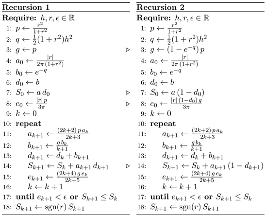
5. Recursion and Asymptotic Speed of Convergence

Let $\tilde{S}=\frac{rS}{2\pi \left(1+r^2\right)}$ and ${\tilde{e}}_k=B_k$ , where S and $B_k$ relate to Theorem 4. Using (34) and (28), the series $\tilde{S}$ can be calculated by Recursion 1 (tildes are omitted). Analogously, let $\hat{S}=\frac{rS}{2\pi \left(1+r^2\right)}$ and ${\hat{e}}_k=B_k$ , where S and $B_k$ relate to Theorem

3. The series $\hat{S}$ can be calculated by Recursion 2 (hats are omitted). In practice, both recursions can be easily combined, since only four steps, marked with $⊳$ , are different.

In both cases, given $\epsilon >0$ , the recursion is terminated when the condition $e_{k+1}<\epsilon$ is met and $S_{k+1}$ is taken as its result. However, if $\epsilon >0$ is too small, or even intentionally negative, the calculation proceeds up to the actual accuracy threshold—the recursion is terminated when the condition $S_{k+1}\le S_k$ is met. This criterion was used in the calculations presented in the next section.

In both recursions, all variables are positive and are bounded upward. If $q\ne 0$ , the sequence $\left\{d_k\right\}$ strictly increases and, due to (24), converges to 1. The sequence $\left\{S_k\right\}$ is strictly increasing if $r\ne 0$ . If $r=0$ , the recursion terminates

with $S_1=0$ . Note that (7) implies $\left|T\left(r\mathrm{,}h\right)\right|\le \frac{\arctan \left|r\right|}{2\pi }$ . If step 7 in Recursion 2 is replaced by $S_0\leftarrow a_0\left(1-d_0\right)-\frac{\arctan \left|r\right|}{2\pi }$ , the sequence $\left\{S_k\right\}$ changes its sign but keeps the direction. However, the modified Recursion 2 computes $\hat{S}=\frac{rS}{2\pi \left(1+r^2\right)}-\frac{\arctan r}{2\pi }$ .

Let ${\tilde{S}}_n$ and ${\hat{S}}_n$ be the results of Recursion 1 and modified Recursion 2 respectively, calculated with the same h and r if $\left|r\right|\le 1$ , or with $\bar{h}$ and $\bar{r}$ if $\left|r\right|>1$ . Let ${\tilde{\Phi }}_{\rho }^2\left(h\mathrm{,0}\right)$ be calculated by (35) or (39), where unknown remainders are ignored. Analogously, let ${\hat{\Phi }}_{\rho }^2\left(h\mathrm{,0}\right)$ be calculated by (30) or (38), where also

$\frac{\arctan r}{2\pi }$ is ignored. If $\left|r\right|\le 1$ , then ${\tilde{\Phi }}_{\rho }^2\left(h\mathrm{,0}\right)\le {\Phi }_{\rho }^2\left(h\mathrm{,0}\right)\le {\hat{\Phi }}_{\rho }^2\left(h\mathrm{,0}\right)$ if $r\ge 0$

and ${\tilde{\Phi }}_{\rho }^2\left(h\mathrm{,0}\right)\ge {\Phi }_{\rho }^2\left(h\mathrm{,0}\right)\ge {\hat{\Phi }}_{\rho }^2\left(h\mathrm{,0}\right)$ if $r<0$ . Even if $\left|r\right|>1$ , one of ${\tilde{\Phi }}_{\rho }^2\left(h\mathrm{,0}\right)$ and ${\hat{\Phi }}_{\rho }^2\left(h\mathrm{,0}\right)$ underestimates and the other overestimates ${\Phi }_{\rho }^2\left(h\mathrm{,0}\right)$ . Consequently, the upper bounds (31) and (36) are not needed if $\tilde{S}$ and modified $\hat{S}$ are calculated in the same recursion which terminates when $\left|{\hat{S}}_{k+1}-{\tilde{S}}_{k+1}\right|$ become small enough. Upper bounds are also not needed if in Recursions 1 and 2 step 17 is replaced so that $S_{k+1}\le S_k$ is the only termination condition. In this case, steps 3, 8 and 15 are unnecessary.

Given q, which one of the series (29) and (34) converges faster? Since $P\left(k+\mathrm{1,}x\right)$ is a cdf of the gamma distribution with the median

$\nu \in \left(k+\frac{2}{3}\mathrm{,}k+1\right)$ , it follows $P\left(k+\mathrm{1,}q\right)\le Q\left(k+\mathrm{1,}q\right)$ if $q\le \nu <k+1$ . The an

swer depends on the number of considered terms, which depends on the prescribed accuracy. On this basis, it seems that series (29) is more suitable than (34) for “small” q and vice versa for “large” q. Table 1 and Table 4 in the next section show how this is reflected in practice.

Gautschi’s inequality $x^{1-s}<\frac{\Gamma \left(x+1\right)}{\Gamma \left(x+s\right)}<{\left(x+1\right)}^{1-s}$ ( [27] , p. 138, 5.6.4) with $s=\frac{1}{2}$ implies $\frac{\sqrt{k\pi }}{2k+1}<\frac{\left(2k\right)!!}{\left(2k+1\right)!!}<\frac{\sqrt{\left(k+1\right)\pi }}{2k+1}$ . Combining it with (25), sending $k\to \infty$ and neglecting non-essential constants imply that the series (29) asymptotically converges as ${\displaystyle {\sum }_k}\frac{q^{k+1}{\text{e}}^{-q}}{\left(k+1\right)\mathrm{<mo>\; !\; </mo>}}\frac{{\rho }^{2k}}{\sqrt{k+1}}$ . Assuming calculation with $\bar{h}$ , $\bar{r}$ and (38) instead of h, r and (30) respectively if $\left|r\right|>1$ , hence ${\rho }^2>\frac{1}{2}$ , and recalling that q is invariant on the transformation of $rh\mapsto \bar{h}$ and $\frac{1}{r}\mapsto \bar{r}$ , we get an asymptotic convergence as ${\displaystyle {\sum }_k}\frac{{\bar{q}}^{k+1}{\text{e}}^{-\bar{q}}}{\left(k+1\right)!}\frac{{\bar{\rho }}^{2k}}{\sqrt{k+1}}={\displaystyle {\sum }_k}\frac{q^{k+1}{\text{e}}^{-q}}{\left(k+1\right)!}\frac{{\left(1-{\rho }^2\right)}^k}{\sqrt{k+1}}$ . The series (29) or its corresponding transformed version, unwritten and based on (40c), asymptotically converges as ${\displaystyle {\sum }_k}\frac{q^{k+1}{\text{e}}^{-q}}{\left(k+1\right)!}\frac{{\left(\min \left\{{\rho }^2,1-{\rho }^2\right\}\right)}^k}{\sqrt{k+1}}={\displaystyle {\sum }_k}\frac{q^{k+1}{\text{e}}^{-q}}{\left(k+1\right)!}\frac{\min \left\{r^{2k},1\right\}}{\sqrt{k+1}{\left(1+r^2\right)}^k}$ , where $q=\frac{1}{2}\left(1+r^2\right)h^2=\frac{h^2}{2\left(1-{\rho }^2\right)}$ . On the other hand, since (24) implies ${\lim }_{k\to \infty }Q\left(k+\mathrm{1,}x\right)=1$ , the series (34) or its corresponding transformed version, unwritten and based on (40d), asymptotically converges as ${\displaystyle {\sum }_k}\frac{{\left(\min \left\{{\rho }^2\mathrm{,1}-{\rho }^2\right\}\right)}^k}{\sqrt{k+1}}={\displaystyle {\sum }_k}\frac{\min \left\{r^{2k}\mathrm{,1}\right\}}{\sqrt{k+1}{\left(1+r^2\right)}^k}$ , hence in the worst case as ${\displaystyle {\sum }_k}\frac{1}{2^k\sqrt{k+1}}$ .

Based on both asymptotic convergences, comparing (34) to (29) would be unfair because the calculation of $\arctan \left|r\right|$ should also be taken into account for (29). Since it is implicitly embedded in Recursion 1, it is calculated on the fly at the cost of worse speed of convergence. Each of the recursions is executable with the basic four arithmetic operations, two calls of elementary functions (if the calculation of r from $\rho$ is also considered), and $\arctan \left|r\right|$ in the modified Recursion 2. However, the computational cost of $\Phi \left(h\right)$ (and $\Phi \left(rh\right)$ if needed) should also be taken in account, but it is the same in (29) and (34).

6. Numeric Issues and Testing Results

A common cause of numerical instability, where two absolutely large values give an absolutely small result when added or subtracted, cannot occur in Recursions 1 and 2. The calculation by them is stable, but something may happen that needs

to be pointed out. The side effect of transforming $rh\mapsto \bar{h}$ and $\frac{1}{r}\mapsto \bar{r}$ is that

$\left|\bar{h}\right|$ can become unusually large. When computing $\Phi \left(h\right)$ , according to Marsaglia ( [28] , p. 2), “[...] the region of interest may not be the statistician’s $0<x<5$ , say, but rather $10<x<14$ [...]’’. Assume the same needs when computing ${\Phi }_{\rho }^2\left(h\mathrm{,0}\right)$ ,

and using transformed parameters if ${\rho }^2>\frac{1}{2}$ . If $h=14$ and

$\rho =\frac{10}{\sqrt{1+{10}^2}}\approx 0.995$ , then $r\approx 10$ , $\bar{r}\approx 0.1$ and $\bar{h}\approx 140$ , implying that the

region of interest could be $\left|h\right|<140$ . Even the usual $\left|h\right|<5$ transformed to $\left|\bar{h}\right|<50$ is well beyond the established limits.

The “problem” of too large $\left|h\right|$ is mentioned because we have to be aware of it if we are going to perform high-precision computation. In any case, the recursion must be complemented by a suitable computation of $\Phi \left(h\right)$ and $\arctan r$ if needed. As an example that not all are like that, the computation by the well

known series $\Phi \left(x\right)=\frac{1}{2}+\frac{1}{\sqrt{2\pi }}{\displaystyle {\sum }_{k=0}^{\infty }}\frac{{\left(-1\right)}^k{x}^{2k+1}}{2^{k}k!\left(2k+1\right)}$ ( [1] , p. 932, 26.2.10) and the

standard double precision arithmetic is numerically unstable even for moderately large $\left|h\right|$ , e.g. using the programming language R [29] , for $h=10$ we get a completely wrong result, approximately −1683. A similar problem can lead to a significant decrease in accuracy if $T\left(h\mathrm{,}r\right)$ is calculated with (7), as will be seen in Subsection 6.1.

In double precision arithmetic, the minimal positive non-zero number is $\eta \approx 2.23\times {10}^{-308}$ . Assuming $b_0={\text{e}}^{-q}\ge \eta$ , it follows $q_{\max }=-\log \left(\eta \right)\approx 708.40$ and

$h_{\max }\left(r\right)=\sqrt{-\frac{2\log \left(\eta \right)}{1+r^2}}$ . If $\left|r\right|\le 1$ , then $h_{\max }\left(r\right)$ is between $h_{\max }\left(1\right)\approx 26.62$ and

$h_{\max }\left(0\right)\approx 37.64$ . If ${\text{e}}^{-q}<\eta$ , then all elements of the sequence $\left\{b_k\right\}$ are zero. Consequently, all elements of $\left\{d_k\right\}$ are one and all elements of $\left\{S_k\right\}$ in Recursion 2 are zero.

From the integral in (7), it follows $\left|T\left(h\mathrm{,}r\right)\right|\le \phi \left(h\right)\frac{\Phi \left(\left|r\right|\left|h\right|\right)-\frac{1}{2}}{\left|h\right|}\le \frac{\phi \left(h\right)}{2\left|h\right|}$ if $h\ne 0$ , where the upper bound is a decreasing function of $\left|h\right|$ . If ${\text{e}}^{-q}<\eta$ and $\left|r\right|\le 1$ , then $\left|h\right|>h_{\max }\left(1\right)$ and $\left|T\left(h,r\right)\right|\le \frac{\phi \left(h_{\max }\left(1\right)\right)}{2h_{\max }\left(1\right)}\approx 1.12\times {10}^{-156}$ . Analogously to the case when $r=0$ , the recursion terminates with $S_1=0$ , which is practically a correct result for $T\left(h\mathrm{,}r\right)$ , as well as ${\Phi }_{\rho }^2\left(h,0\right)=\frac{1}{2}$ if $h>0$ , and ${\Phi }_{\rho }^2\left(h,0\right)=0$ if $h<0$ .

The Recursions 1 and 2 with adjustment of their results according to (40a)—(40d) are implemented in the package Phi2rho [30] . It contains the functions OwenT(), hereafter Phi2rho::OwenT(), and Phi2xy(), which compute $T\left(h\mathrm{,}r\right)$ and ${\Phi }_{\rho }^2\left(x\mathrm{,}y\right)$ respectively. They also enable computation with the tetrachoric and Vasicek’s series, original or accelerated. The latter means that h and r are transformed if $r>1$ and $r<1$ for the tetrachoric and Vasicek’s series respectively, and the Equation (15) is used, so (18) instead of (9) in the case of tetrachoric series. For the sake of comparison, all series were considered during testing in Subsection 6.1. In Subsection 6.2, the original tetrachoric and Vasicek’s series were excluded because they converge too slowly for unfavorable $\rho$ .

During testing, the values of $T\left(r\mathrm{,}h\right)$ and ${\Phi }_{\rho }^2\left(x\mathrm{,}y\right)$ were computed for a selected and randomly generated set of parameters. Reference values were computed using the accelerated tetrachoric series and quadruple (128-bit) precision. Absolute differences between tested and reference values are declared as absolute errors. The maximum absolute error is considered a measure of accuracy. Since the mean values and some quantiles are also important, they are shown in the tables in Subsection 6.2. An integral part of the testing was also a comparison of the results obtained with the Phi2rho package and competing packages available on CRAN.

6.1. Numeric Issues and Results When Computing $T\left(h,r\right)$

Numerical calculations of $T\left(h\mathrm{,}r\right)$ were performed on 39,999 grid points $\left(h\mathrm{,}r\right)$ ,

where h ranges from −10 to 10 in increments of 0.1, $r=\frac{\rho }{\sqrt{1-{\rho }^2}}$ and $\rho$ ranges

from −0.99 to 0.99 in increments of 0.01. Since for $\rho =\pm 0.99$ we get $r\approx \pm 7$ , the actual range of h for which $\Phi \left(h\right)$ must be computed is approximately from −70 to 70, so well beyond the $h_{\max }\left(0\right)\approx 37.64$ .

Note atanExt = no in tables means that Recursion 1 was executed, hence (40b) was used if $\left|r\right|\le 1$ and (40d) if $\left|r\right|>1$ , and atanExt = yes means that Recursion 2 was executed, hence (40a) was used if $\left|r\right|\le 1$ and (40c) if $\left|r\right|>1$ . Both recursions are well suited for vectors, so each of the parameters h and r can be a scalar or a vector. If they are both vectors, they must be of the same length, if one of h and r is a vector and the other is a scalar, the latter is replicated to the length of the former. Since the number of iterations is determined by the “worst’’ component, we would expect execution to be faster if function calls are done in a loop for each component of the vector separately, but usually the run time is significantly increased due to the overhead of the loop, more initialization, etc.

For the consistency test, $T\left(h\mathrm{,}r\right)$ was calculated on the test grid with h and r both scalars, one a scalar and the other a vector. For all three calculations with Recursion 1, the results matched perfectly, as well as for all three with Recursion 2. The maximum absolute difference between calculations with Recursions 1 and 2 was approximately 9.49 × 10⁻¹⁷.

When testing accuracy, the tetrachoric and Vasicek’s series, original and accelerated, were also tested, using $T\left(h,r\right)={\Phi }_{\rho }^2\left(h,0\right)-\frac{1}{2}\Phi \left(h\right)$ . By transforming the

parameters, if appropriate, both comparison methods gained a lot, as can be concluded from Table 1. The absolute errors, the maximum values of which are

Table 1. Double precision computation of $T\left(h,r\right)={\Phi }_{\rho }^2\left(h,0\right)-\frac{1}{2}\Phi \left(h\right)$ on the test grid.

collected in this table, were calculated against the reference values computed with the accelerated tetrachoric series and 128-bit precision.

Since the vector computations were performed, there are two average numbers of iterations. The first is empirical because the iterations were terminated according to the “worst’’ component of the vector, and the second is hypothetical, if the computations were performed for each component separately. Since all iterations ran to the accuracy limit and with an unbounded number of iterations, the original Vasicek’s series needed the enormous number of iterations, not only for the worse case, but also in average, when calculating with scalar h and vector

r. However, it is not intended for cases with ${\rho }^2<\frac{1}{2}$ , and its error can be well estimated, which was ignored here.

Comparative computations with competing packages were also performed on

the test grid, using $T\left(h,r\right)={\Phi }_{\rho }^2\left(h,0\right)-\frac{1}{2}\Phi \left(h\right)$ . The pbinorm() function from

the VGAM package [15] , i.e. using (7), had an average and maximum absolute error of 1.12 × 10⁻⁸ and 3.62 × 10⁻⁷ respectively. Similar maximum absolute errors were obtained by the function pbvnorm() from the pbv package [31] , which is based on [6] , and pmvnorm() from the mvtnorm package, but only with the parameter algorithm = Miwa.

6.2. Numeric Issues and Results When Computing ${\Phi }_{\rho }^2\left(x,y\right)$

In all ${\Phi }_{\rho }^2\left(x,y\right)$ computational methods based on (4) and (5), or (13) and (14), exceptional cases with $\left|\rho \right|=1$ , $x\ne 0$ and $x-y\mathrm{sgn}\left(\rho \right)=0$ are not problematic because (3) can be used, however, nearby cases are their weak point. Recalling

that $q_x=q_y=\frac{x^2-2\rho xy+y^2}{2\left(1-{\rho }^2\right)}=q$ and using (10) and (2), it follows $\frac{\partial }{\partial \rho }{\Phi }_{\rho }^2\left(x,y\right)=\frac{{\text{e}}^{-q}}{2\pi \sqrt{1-{\rho }^2}}$ and ${\lim }_{\left|\rho \right|\to 1}\frac{\partial }{\partial \rho }{\Phi }_{\rho }^2\left(x,y\right)=0$ , except if

$x-y\mathrm{sgn}\left(\rho \right)=0$ . If $\left|\rho \right|$ is close to 1 and $x-y\mathrm{sgn}\left(\rho \right)\simeq 0$ , then

$x^2-2\rho xy+y^2\simeq 0$ and q may be small enough that $\frac{\partial }{\partial \rho }{\Phi }_{\rho }^2\left(x\mathrm{,}y\right)$ is moderate

or even large. As a result, even a small rounding error in the calculation of key variables that depend on $\rho$ can cause a much larger error in the result. The calculation of $r_x$ and $r_y$ with (14) is particularly problematic. In a similar situation, Meyer ( [9] , p. 5) recommends an equivalent but less sensitive calculation

by $r_x=\frac{x-y}{x\sqrt{1-{\rho }^2}}-\sqrt{\frac{1-\rho }{1+\rho }}$ if $\rho \approx 1$ and $r_x=\frac{x+y}{x\sqrt{1-{\rho }^2}}-\sqrt{\frac{1+\rho }{1-\rho }}$ if $\rho \approx -1$ , and

analogously for $r_y$ . In our case, his proposal improves accuracy, but does not solve the problem sufficiently.

The problem could be solved by a hybrid computation along the lines of some other methods, e.g. the series from ( [32] , pp. 242-245) could be used if $\left|\rho \right|\approx 1$ and $x-y\mathrm{sgn}\left(\rho \right)\simeq 0$ . Using the initial idea to develop these series, i.e. axis rotation in a way that removes the cross product term $-2\rho st$ in (1), by setting

$s=\frac{u+v}{\sqrt{2}}$ and $t=\frac{u-v}{\sqrt{2}}$ the Equation (1) transforms to

$\begin{array}{c}{\Phi }_{\rho }^2\left(x\mathrm{,}y\right)=\frac{1}{2\pi \sqrt{1-{\rho }^2}}{\displaystyle {\int }_{-\infty }^{\frac{x-y}{\sqrt{2}}}}{\text{e}}^{-\frac{u^2}{2\left(1-\rho \right)}}\left({\displaystyle {\int }_{-\infty }^{u+\sqrt{2}y}}{\text{e}}^{-\frac{v^2}{2\left(1+\rho \right)}}\text{d}v\right)\text{d}u\\ +\frac{1}{2\pi \sqrt{1-{\rho }^2}}{\displaystyle {\int }_{\frac{x-y}{\sqrt{2}}}^{\infty }}{\text{e}}^{-\frac{u^2}{2\left(1-\rho \right)}}\left({\displaystyle {\int }_{-\infty }^{-u+\sqrt{2}x}}{\text{e}}^{-\frac{v^2}{2\left(1+\rho \right)}}\text{d}v\right)\text{d}u\end{array}$

and, using $\frac{u}{\sqrt{1-\rho }}=\tilde{u}$ and $\frac{v}{\sqrt{1+\rho }}=\tilde{v}$ , to

$\begin{array}{c}{\Phi }_{\rho }^2\left(x\mathrm{,}y\right)={\displaystyle {\int }_{-\infty }^{\frac{x-y}{\sqrt{2\left(1-\rho \right)}}}}\phi \left(\tilde{u}\right)\Phi \left(\tilde{u}\sqrt{\frac{1-\rho }{1+\rho }}+y\sqrt{\frac{2}{1+\rho }}\right)\text{d}\tilde{u}\\ +{\displaystyle {\int }_{\frac{x-y}{\sqrt{2\left(1-\rho \right)}}}^{\infty }}\phi \left(\tilde{u}\right)\Phi \left(-\tilde{u}\sqrt{\frac{1-\rho }{1+\rho }}+x\sqrt{\frac{2}{1+\rho }}\right)\text{d}\tilde{u}\mathrm{.}\end{array}$

By transforming $\tilde{u}\mapsto -\tilde{u}$ in the second integral and using ( [14] , p. 402, 10,010.1),

it follows ${\Phi }_{\rho }^2\left(x\mathrm{,}y\right)={\Phi }_{{\rho }^{\mathrm{<mo>\; *\; </mo>}}}^2\left(\frac{x-y}{\sqrt{2\left(1-\rho \right)}}\mathrm{,}y\right)+{\Phi }_{{\rho }^{\mathrm{<mo>\; *\; </mo>}}}^2\left(-\frac{x-y}{\sqrt{2\left(1-\rho \right)}}\mathrm{,}x\right)$ , where ${\rho }^{\mathrm{<mo>\; *\; </mo>}}=-\sqrt{\frac{1-\rho }{2}}$ . This equation is suitable for $\rho \approx 1$ . From it and ${\Phi }_{\rho }^2\left(x\mathrm{,}y\right)=\Phi \left(x\right)-{\Phi }_{-\rho }^2\left(x\mathrm{,}-y\right)$ we obtain the equation

${\Phi }_{\rho }^2\left(x\mathrm{,}y\right)=\Phi \left(x\right)-{\Phi }_{\hat{\rho }}^2\left(\frac{x+y}{\sqrt{2\left(1+\rho \right)}}\mathrm{,}-y\right)-{\Phi }_{\hat{\rho }}^2\left(-\frac{x+y}{\sqrt{2\left(1+\rho \right)}}\mathrm{,}x\right)\mathrm{,}$

where $\hat{\rho }=-\sqrt{\frac{1+\rho }{2}}$ , that is suitable for $\rho \approx -1$ . Both are combined in

${\Phi }_{\rho }^2\left(x,y\right)=\frac{1-\mathrm{sgn}\left(\rho \right)}{2}\Phi \left(x\right)+\mathrm{sgn}\left(\rho \right)\left({\Phi }_{\tilde{\rho }}^2\left(z,\tilde{y}\right)+{\Phi }_{\tilde{\rho }}^2\left(-z,x\right)\right),$ (41)

where $\tilde{\rho }=-\sqrt{\frac{1-\left|\rho \right|}{2}}$ , $\tilde{y}=y\mathrm{sgn}\left(\rho \right)$ and $z=\frac{x-\tilde{y}}{\sqrt{2\left(1-\left|\rho \right|\right)}}$ . Noting that

$\tilde{q}=\frac{{\tilde{y}}^2-2\tilde{\rho }\tilde{y}z+z^2}{2\left(1-{\tilde{\rho }}^2\right)}=\frac{x^2+2\tilde{\rho }xz+z^2}{2\left(1-{\tilde{\rho }}^2\right)}=\frac{x^2-2\rho xy+y^2}{2\left(1-{\rho }^2\right)}=q,$

hence ${\phi }_{\tilde{\rho }}^2\left(z,\tilde{y}\right)={\phi }_{\tilde{\rho }}^2\left(-z,x\right)=\frac{{\text{e}}^{-q}}{\pi \sqrt{2\left(1+\left|\rho \right|\right)}}$ , we stop here because one potentially critical case is replaced with two non-critical ones.

If we continued to simplify the right side of (41) by (13), we would get (13). This actually happens when calculating with the functions used in tests, but it turns out that the results are more accurate than if we start with (13) if $\left|\rho \right|\approx 1$ and $x-y\mathrm{sgn}\left(\rho \right)\simeq 0$ . Of course, the Equation (41) could be used as a starting point instead of (13) in all cases, but this is not rational because it requires 4 calculations of the T function instead of 2, two of which cancel each other out, at least in theory, and as a result, in non-critical cases the error may be larger than when starting with (13). When testing, (41) was used as a starting point instead

of (13) if ${\phi }_{\rho }^2\left(x,y\right)>1$ . However, since $\min \left\{\left|\rho \right|\mathrm{,}\sqrt{\frac{1-\left|\rho \right|}{2}}\right\}\le \frac{1}{2}$ , using (41) may

also make sense in some other circumstances, e.g. when computing directly with (8).

In this case, testing was performed on the randomly generated set of parameters. After setting the random generator seed to 123 to allow replication and independent verification, one million x values, one million y values, and one million ρ values were drawn from a uniform distribution on the intervals $\left(-\mathrm{10,10}\right)$ , $\left(-\mathrm{10,10}\right)$ , and $\left(-\mathrm{1,1}\right)$ respectively.

For each triplet $\left(x\mathrm{,}y\mathrm{,}\rho \right)$ , auxiliary values $q=\frac{x^2-2\rho xy+y^2}{2\left(1-{\rho }^2\right)}$ and

${\phi }_{\rho }^2\left(x\mathrm{,}y\right)=\frac{{\text{e}}^{-q}}{2\pi \sqrt{1-{\rho }^2}}$ were calculated. For the new series, the tested ${\Phi }_{\rho }^2\left(x\mathrm{,}y\right)$

values were computed using (41) as a branch point and (13) for both branches if ${\phi }_{\rho }^2\left(x,y\right)>1$ , and using (13) directly otherwise. The same applies for the tetrachoric and Vasicek’s series, only (4) must be used instead of (13). However, the described procedure is built in the Phi2xy() function. The tested ${\Phi }_{\rho }^2\left(x\mathrm{,}y\right)$ values needed for the preparation of Table 2 were computed with:

row 1: Phi2xy(x, y, ρ, fun = "tOwenT");

row 2: Phi2xy(x, y, ρ, fun = "vOwenT");

row 3: Phi2xy(x, y, ρ, fun = "mOwenT", opt = FALSE);

row 4: Phi2xy(x, y, ρ, fun = "mOwenT", opt = TRUE).

The absolute errors, which statistics are collected in Table 2, were calculated against reference values computed with the accelerated tetrachoric series as described, but with 128-bit precision. From a user’s point of view, only the parameters x, y and ρ needed to be converted into 128-bit “mpfr-numbers’’ before calling Phi2xy(x, y, ρ, fun = "tOwenT"), hence x <- mpfr(x, precBits = 128) and analogously for y and ρ. In this case, the computation took significantly more time, since all intermediate and final results were 128-bit “mpfr-numbers’’.

In this test, ${\rho }_{\min }\approx -0.99999991$ , ${\rho }_{\max }\approx 0.99999775$ , there are 5 cases with ${\phi }_{\rho }^2\left(x,y\right)>1$ and $\max {\phi }_{\rho }^2\left(x\mathrm{,}y\right)\approx 1.38$ .

In order to better check the accuracy if $\left|\rho \right|$ is close to 1, the computation was repeated with the same x and y, and ${\rho }^{\mathrm{<mo>\; *\; </mo>}}=2\Phi \left(8\rho \right)-1$ . In this case, more than half of $\left|{\rho }^{\mathrm{<mo>\; *\; </mo>}}\right|$ are greater than 0.9999 and none is equal to 1. The results are in Table 3.

In this test, there are 178 cases with ${\phi }_{\rho }^2\left(x,y\right)>1$ and $\max {\phi }_{\rho }^2\left(x\mathrm{,}y\right)\approx 376$ . For both novel series in Table 3, the maximum absolute error is 1.54 × 10⁻¹⁴ if (41) is not used, improving to 1.21 × 10⁻¹⁵ if Meyer’s advice is followed. Similarly applies to the other two series.

Table 2. ${\Phi }_{\rho }^2\left(x\mathrm{,}y\right)$ computation—absolute error comparison.

Table 3. ${\Phi }_{{\rho }^{\mathrm{<mo>\; *\; </mo>}}}^2\left(x\mathrm{,}y\right)$ computation—absolute error comparison.

Due to the time-consuming 128-bit precision computation, the presented tests are the only performed tests based on the 128-bit precision reference values. However, additional tests were made by comparing the results of Phi2xy() with the results obtained by other functions from packages available on CRAN. For three functions, the accuracy was found to be worse than 2 × 10⁻⁷ as measured by the maximum absolute error on the test grid from Subsection 6.1. Regarding accuracy, only the function pmvnorm() with the parameter algorithm = TVPACK from the mvtnorm package proved to be equivalent to Phi2xy() and even slightly more accurate with the maximum absolute errors 2.58 × 10⁻¹⁶ and 2.19 × 10⁻¹⁶ on the test sets of triplets $\left(x\mathrm{,}y\mathrm{,}\rho \right)$ and $\left(x\mathrm{,}y\mathrm{,}{\rho }^{\mathrm{<mo>\; *\; </mo>}}\right)$ respectively. The same function with algorithm = GenzBretz achieved 2.58 × 10⁻¹⁶ and 2.20 × 10⁻¹¹.

The OwenQ::OwenT() function also proved to be equivalent to Phi2xy() as measured by the maximum absolute error on the test sets of triplets, but only when upgraded to compute ${\Phi }_{\rho }^2\left(x\mathrm{,}y\right)$ in the manner used in Phi2xy(). This function and Phi2rho::OwenT() are essentially wrappers for the internal functions tOwenT(), vOwenT() and mOwenT(), which as workhorses compute series.

In terms of reliability, stability and accuracy of the new methods, no problems or significant differences according to the parameters from the different data sets were detected, except those already described and related to $\left|\rho \right|\approx 1$ and $x-y\mathrm{sgn}\left(\rho \right)\simeq 0$ . To eliminate them, the Equation (44) was derived, which also proved to be successful when using the OwenQ::OwenT() function, upgraded to compute ${\Phi }_{\rho }^2\left(x\mathrm{,}y\right)$ . Regarding parameters from different data sets, the only detected big difference is in the number of iterations, as can be seen from Figure 1.

Two million ${\Phi }_{\rho }^2\left(x\mathrm{,}y\right)$ computations on Windows 10 and 64-bit R 4.3.1 on the old Intel i7-6500U CPU @ 2.50 GHz and 8 GB RAM, using only one thread

Figure 1. $T\left(h,r\right)$ computation with the new series (atanExt = yes) with double (left) and 128-bit (right) precision—number of iterations.

of four, lasted 26, 31 and 286 seconds for Phi2xy(), upgraded OwenQ::OwenT() and pmvnorm() with algorithm = TVPACK respectively. The 128-bit precision reference values computation took over 17 hours, compared to 43 seconds for the double precision one. Based on Table 1 and Table 4, we can conclude that the increased number of iterations has only an insignificant effect on the huge time extension factor.

6.3. High-Precision Computation

All functions in the Phi2rho package are ready to use the Rmpfr package, which enables using arbitrary precision numbers instead of double precision ones and provides all the high-precision functions needed. It interfaces R to the widely used C Library MPFR [33] . Assuming that the Rmpfr package is loaded, the functions should only be called with the parameters, which are “mpfr-numbers’’ of the same precision. All 128-bit precision benchmark values used in Subsections 6.1 and 6.2 were calculated using Rmpfr.

To get a sense of how the number of iterations depends on the required precision, the test from Subsection 6.1 was partially repeated using the 128-bit precision computation. The results are collected in Table 4. Note that $2^{-128}\approx 2.94\times {10}^{-39}$ and that in this case the values in the table are not the maximum absolute errors because the comparison values are computed with the same precision.

From Table 1 and Table 4 can be concluded that there is no significant difference in accuracy between the compared series if the accelerated series are considered, but one of the new series converges significantly faster than the others. It can also be concluded that the Vasicek’s series with $\bar{\rho }$ instead of $\rho$ is a

reasonable alternative to the tetrachoric series (8) also for ${\rho }^2<\frac{1}{2}$ and remains a reasonable alternative for ${\rho }^2>\frac{1}{2}$ if compared to the transformed tetrachoric series (9).

Table 4. 128-bit precision computation of $T\left(h,r\right)={\Phi }_{\rho }^2\left(h,0\right)-\frac{1}{2}\Phi \left(h\right)$ on the test grid.

Table 5. A special case of high-precision computing—absolute error comparison.

The number of iterations for the computation with the new series with double and 128-bit precision can be compared in Figure 1. Only the first quadrant is presented because others are its mirror images.

We also provide examples with $r=1$ and $r=-1$ for which reference values can be computed alternatively. $A={\Phi }_{\sqrt{2}\mathrm{<mo>\; /\; </mo>2}}^2\left(\mathrm{2.1,0}\right)$ and $B={\Phi }_{-\sqrt{2}\mathrm{<mo>\; /\; </mo>2}}^2\left(\mathrm{2.1,0}\right)$ were computed by (13) and (14), and by the right side of (16) by the pnorm() function from the package Rmpfr as a benchmark. In all cases, the latter was computed by double the precision expressed in bits and used for the former. Both reference values were used to compare how quickly the compared series converge when computing with more than 128-bit precision. In Table 5 and Table 6, for each of them the absolute error and the number of iterations, which is the same for both computations, is presented. Since $\left|r\right|=1$ , there is no difference between the original and accelerated tetrachoric series, and the same applies to Vasicek’s series.

Time-consuming high precision testing was less intensive than double precision one. Since there is no competing package on CRAN ready for high-precision computation of ${\Phi }_{\rho }^2\left(x\mathrm{,}y\right)$ , it could not be supplemented by comparison computations with competing packages.

Table 6. A special case of high-precision computing—absolute error comparison.

7. Conclusions

If the generally applicable Theorem 2 is not considered, Theorems 3 and 4, and Corollary 2 are interesting mainly theoretically, because Theorem 5, together with (13) and (14), replaces and supplements them in practice. The series (40a)—(40d) enable fast and numerically stable computation, which is often more important than the speed of convergence. From Table 1 and Table 4 can be concluded that the computation with (40a) or (40c) needs significantly fewer iterations than the computation with the accelerated tetrachoric and Vasicek’s series, and from Table 5 and Table 6 can be assumed that the advantage increases with increasing precision. For 53-bit precision (double precision), it required a half, and for 1024-bit precision only a fifth, of the iterations demanded by the competing series. However, the cost of calculating $\arctan r$ is not taken into account. In connection with this, let us just mention two more questions.

Recalling that ${\text{e}}^{-x}{I}_n\left(x\right)=P\left(n+\mathrm{1,}x\right)$ , the Taylor series of the arctangent function and (7) imply

$\begin{array}{c}T\left(h\mathrm{,}r\right)=\frac{\arctan r}{2\pi }-\frac{1}{2\pi }{\displaystyle \underset{k=0}{\overset{\infty }{\sum }}}\frac{{\left(-1\right)}^k{r}^{2k+1}}{2k+1}P\left(k+\mathrm{1,}\frac{1}{2}{h}^2\right)\\ =\frac{1}{2\pi }{\displaystyle \underset{k=0}{\overset{\infty }{\sum }}}\frac{{\left(-1\right)}^k{r}^{2k+1}}{2k+1}Q\left(k+\mathrm{1,}\frac{1}{2}{h}^2\right)\mathrm{,}\end{array}$

which Fayed and Atiya ( [32] , p. 241) have already noticed. If the above series, (29) and (34) are viewed as functions of the variable h, they have a similar structure, but the coefficients, depending on r, belong to different arctangent series. Whether the similarity could be explained by a similar Euler transform as the one which transforms the Taylor arctangent series to the Euler’s arctangent series seems interesting question, but was not deeply explored.

In Recursion 1, the external calculation of the arctangent function is avoided, assuming that the Euler’s series (19) is used for it, and the expectation that there would be no difference in the number of iterations for Recursions 1 and 2 if those for calculating the arctangent were also taken into account. However, the use of the external arctangent calculation allows the use of already known and possible future faster converging series. Such is the case with

$\arctan r=\frac{r}{\sqrt{1+r^2}}{\displaystyle \underset{k=0}{\overset{\infty }{\sum }}}\frac{\left(2k-1\right)!!}{\left(2k\right)!!\left(2k+1\right)}{\left(\frac{r^2}{1+r^2}\right)}^k\left(r\in ℝ\right),$ (42)

which is based on the Taylor series of $\arcsin r$ and $\arctan r=\arcsin \frac{r}{\sqrt{1+r^2}}$ .

Indeed, the number of iterations is not significantly smaller if $\left|r\right|\le 1$ and the accuracy obtained by double precision computation is sufficient, and even the square root must be calculated, but it could be significantly smaller in high-precision computation. The Euler’s series (19) is included in [1] and [27] , but (42) is not, even though it converges faster. It can be found in ( [22] , p. 61, 1.644 1.) as

$\arctan r=\frac{r}{\sqrt{1+r^2}}{\displaystyle \underset{k=0}{\overset{\infty }{\sum }}}\frac{(2k)!}{2^{2k}{\left(k!\right)}^2\left(2k+1\right)}{\left(\frac{r^2}{1+r^2}\right)}^k$

with a reference to the 1922 source. Due to equations $\left(2k-1\right)\mathrm{<mo>\; !\; </mo>\; <mo>\; !\; </mo>}=\frac{\left(2k\right)\mathrm{<mo>\; !\; </mo>}}{2^{k}k\mathrm{<mo>\; !\; </mo>}}$ and

$\left(2k\right)\mathrm{<mo>\; !\; </mo>\; <mo>\; !\; </mo>}=2^{k}k\mathrm{<mo>\; !\; </mo>}$ , the coefficients are the same as those in (42). Whether we could also find a corresponding series for the Owen’s T function, which would converge faster than (40b), remains an open challenge.

Conflicts of Interest

The author declares no conflicts of interest regarding the publication of this paper.

References

[1]	Abramowitz, M. and Stegun, I.A. (1972) Handbook of Mathematical Functions. 9th Edition, Dover Publications, Inc., New York.
[2]	Gupta, S.S. (1963) Bibliography on the Multivariate Normal Integrals and Related Topics. The Annals of Mathematical Statistics, 34, 829-838. https://doi.org/10.1214/aoms/1177704005
[3]	Donnelly, T.G. (1973) Algorithm 462: Bivariate Normal Distribution. Communications of the ACM, 16, 638. https://doi.org/10.1145/362375.362414
[4]	Owen, D.B. (1956) Tables for Computing Bivariate Normal Probabilities. The Annals of Mathematical Statistics, 27, 1075-1090. https://doi.org/10.1214/aoms/1177728074
[5]	Divgi, D.R. (1979) Calculation of Univariate and Bivariate Normal Probability Functions. The Annals of Statistics, 7, 903-910. https://doi.org/10.1214/aos/1176344739
[6]	Drezner, Z. and Wesolowsky, G.O. (1990) On the Computation of the Bivariate Normal Integral. Journal of Statistical Computation and Simulation, 35, 101-107. https://doi.org/10.1080/00949659008811236
[7]	Patefield, M. and Tandy, D. (2000) Fast and Accurate Calculation of Owen’s T Function. Journal of Statistical Software, 5, 1-25. https://doi.org/10.18637/jss.v005.i05
[8]	Genz, A. (2004) Numerical Computation of Rectangular Bivariate and Trivariate Normal and t Probabilities. Statistics and Computing, 14, 251-260. https://doi.org/10.1023/B:STCO.0000035304.20635.31
[9]	Meyer, C. (2013) Recursive Numerical Evaluation of the Cumulative Bivariate Normal Distribution. Journal of Statistical Software, 52, 1-14. https://doi.org/10.18637/jss.v052.i10
[10]	Fayed, H.A. and Atiya, A.F. (2014) A Novel Series Expansion for the Multivariate Normal Probability Integrals Based on Fourier Series. Mathematics of Computation, 83, 2385-2402. https://doi.org/10.1090/S0025-5718-2014-02844-5
[11]	Terza, J.V. and Welland, U. (1991) A Comparison of Bivariate Normal Algorithms. Journal of Statistical Computation and Simulation, 39, 115-127. https://doi.org/10.1080/00949659108811343
[12]	Gai, J. (2001) A Computational Study of the Bivariate Normal Probability Function. Master’s Thesis, Queen’s University, Kingston.
[13]	Ağca, Ş.A. and Chance, D.M. (2003) Speed and Accuracy Comparison of Bivariate Normal Distribution Approximations for Option Pricing. The Journal of Computational Finance, 6, 61-96. https://doi.org/10.21314/JCF.2003.102
[14]	Owen, D.B. (1980) A Table of Normal Integrals. Communications in Statistics—Simulation and Computation, 9, 389-419. https://doi.org/10.1080/03610918008812164
[15]	Yee, T.W. (2023) VGAM: Vector Generalized Linear and Additive Models, R Package Version 1.1-8. https://CRAN.R-project.org/package=VGAM
[16]	Laurent, S. (2023) OwenQ: Owen Q-Function, R Package Version 1.0.7. https://CRAN.R-project.org/package=OwenQ
[17]	Genz, A. and Bretz, F. (2009) Computation of Multivariate Normal and t Probabilities. Lecture Notes in Statistics, Springer-Verlag, Heidelberg. https://doi.org/10.1007/978-3-642-01689-9
[18]	Maechler, M. (2023) Rmpfr: R MPFR—Multiple Precision Floating-Point Reliable, R Package Version 0.9-3. https://CRAN.R-project.org/package=Rmpfr
[19]	Kendall, M.G. (1941) Proof of Relations Connected with the Tetrachoric Series and Its Generalization. Biometrika, 32, 196-198. https://doi.org/10.1093/biomet/32.2.196
[20]	Vasicek, O.A. (1998) A Series Expansion for the Bivariate Normal Integral. The Journal of Computational Finance, 1, 5-10. https://doi.org/10.21314/JCF.1998.015
[21]	Plackett, R.L. (1954) A Reduction Formula for Normal Multivariate Integrals. Biometrika, 41, 351-360. https://doi.org/10.1093/biomet/41.3-4.351
[22]	Gradshteyn, I.S. and Ryzhik, I.M. (2015) Table of Integrals, Series, and Products. 8th Edition, Academic Press, Amsterdam.
[23]	Alzer, H. (1997) On Some Inequalities for the Incomplete Gamma Function. Mathematics of Computation, 66, 771-778. https://doi.org/10.1090/S0025-5718-97-00814-4
[24]	Gautschi, W. (1998) The Incomplete Gamma Functions since Tricomi. In: Tricomi’s Ideas and Contemporary Applied Mathematics, Atti Convegni Lincei, Vol. 147, Accademia Nazionale dei Lincei, Rome, 203-237.
[25]	Mitrinović, D.S. (1970) Analytic Inequalities. Springer-Verlag, Berlin. https://doi.org/10.1007/978-3-642-99970-3
[26]	Alzer, H. (1998) Inequalities for the Chi Square Distribution Function. Journal of Mathematical Analysis and Applications, 223, 151-157. https://doi.org/10.1006/jmaa.1998.5965
[27]	Olver, F.W.J., Lozier, D.W., Boisvert, R.F. and Clark C.W. (2010) NIST Handbook of Mathematical Functions. National Institute of Standards and Technology & Cambridge University Press, Cambridge.
[28]	Marsaglia, G. (2004) Evaluating the Normal Distribution. Journal of Statistical Software, 11, 1-11. https://doi.org/10.18637/jss.v011.i04
[29]	R Core Team (2023) R: A Language and Environment for Statistical Computing. R Foundation for Statistical Computing, Vienna. https://www.R-project.org/
[30]	Komelj, J. (2023) Phi2rho: Owen’s T Function and Bivariate Normal Integral, R Package Version 1.0. https://CRAN.R-project.org/package=Phi2rho
[31]	Robitzsch, A. (2020) pbv: Probabilities for Bivariate Normal Distribution, R Package Version 0.4-22. https://CRAN.R-project.org/package=pbv
[32]	Fayed, H.A. and Atiya, A.F. (2014) An Evaluation of the Integral of the Product of the Error Function and the Normal Probability Density with Application to the Bivariate Normal Integral. Mathematics of Computation, 83, 235-250. https://doi.org/10.1090/S0025-5718-2013-02720-2
[33]	Fousse, L., Hanrot, G., Lefèvre, V., Pélissier, P. and Zimmermann, P. (2007) MPFR: A Multiple-Precision Binary Floating-Point Library with Correct Rounding. ACM Transactions on Mathematical Software, 33, 13-es. https://doi.org/10.1145/1236463.1236468