On Topics in Quantum Games

Yshai Avishai^1,2

¹Department of Physics, Ben-Gurion University of the Negev, Beer-Sheva, Israel.
²Yukawa Institute for Theoretical Physics, Kyoto, Japan.

DOI: 10.4236/jqis.2023.133006                

Abstract

This work concentrates on simultaneous move non-cooperating quantum games. Part of it is evidently not new, but it is included for the sake self consistence, as it is devoted to introduction of the mathematical and physical grounds of the pertinent topics, and the way in which a simple classical game is modified to become a quantum game (a procedure referred to as a quantization of a classical game). The connection between game theory and information science is briefly stressed, and the role of quantum entanglement (that plays a central role in the theory of quantum games), is exposed. Armed with these tools, we investigate some basic concepts like the existence (or absence) of a pure strategy and mixed strategy Nash equilibrium and its relation with the degree of entanglement. The main results of this work are as follows: 1) Construction of a numerical algorithm based on the method of best response functions, designed to search for pure strategy Nash equilibrium in quantum games. The formalism is based on the discretization of a continuous variable into a mesh of points, and can be applied to quantum games that are built upon two-players two-strategies classical games, based on the method of best response functions. 2) Application of this algorithm to study the question of how the existence of pure strategy Nash equilibrium is related to the degree of entanglement (specified by a continuous parameter γ ). It is shown that when the classical game G_C has a pure strategy Nash equilibrium that is not Pareto efficient, then the quantum game G_Q with maximal entanglement (γ = π/2) has no pure strategy Nash equilibrium. By studying a non-symmetric prisoner dilemma game, it is found that there is a critical value 0<γ_c<π/2 such that for γ<γ_c there is a pure strategy Nash equilibrium and for γ≥γ_c there is no pure strategy Nash equilibrium. The behavior of the two payoffs as function of γ starts at that of the classical ones at (D, D) and approaches the cooperative classical ones at (C, C) (C = confess, D = don’t confess). 3) We then study Bayesian quantum games and show that under certain conditions, there is a pure strategy Nash equilibrium in such games even when entanglement is maximal. 4) We define the basic ingredients of a quantum game based on a two-player three strategies classical game. This requires the introduction of trits (instead of bits) and quantum trits (instead of quantum bits). It is proved that in this quantum game, there is no classical commensurability in the sense that the classical strategies are not obtained as a special case of the quantum strategies.

Keywords

Two-Players Two Strategies Quantum Game and SU(2) Strategies, Relevance of Entanglement and Bell States, Nash Equilibrium and Its Relation to Entanglement in Pure and Mixed Strategy Quantum Games, Nash Equilibrium and Partial Entanglement, Nash Equilibrium Despite Maximal Entanglement, Two Players Three Strategies Quantum Games: Qutrits and SU(3) Strategies

1. Introduction

The subject matter in the present work is focused on the topic of quantum games, (especially, quantum games based on simultaneous non-cooperative games with two players and two or three strategies for each player), that is an emergent sub-discipline of physics and mathematics. The main effort is directed on the elucidation of Nash equilibrium in quantum games with full information and in games with incomplete information (Bayesian games).

The science of quantum games has been developed rapidly in recent years, together with other similar fields, in particular quantum information to which it is intimately related. As already stressed, the first few sections are not new but included for the sake of self consistence and proper notations.

Quantum game theory models the behavior of strategic agents (players) with access to quantum tools for controlling their strategies. The simplest example is to envision a classical (ordinary) two-player two-strategies game G_C (e.g the prisoner dilemma with two strategies C = confess and D = don’t confess) given in its normal form (a table of payoff functions). In this game, each player communicates with the referee within a “classical” protocol by telling the referee if he confesses or does not confess. One can then quantize G_C to get a quantum game G_Q in which the players communicate with the referee via a specific quantum protocol. The novel elements in this scheme consist of three concepts. First, instead of the four possible positions (CC), (CD), (DC) and (DD), there are an infinitely continuous number of positions represented as different quantum mechanical states (wave functions). Second, instead of the two-point strategy space of each player, there is an infinitely continuous number of new strategies (this should not be confused with mixed strategies). Third, the payoff system is entirely different, as it is based on extracting real numbers from a quantum state that is generically a vector of complex numbers. The fourth difference is the occurrence of quantum entanglement, a conceptually and crucially important new factor that has no analog in standard (classical) game theory. Its significance in quantum game theory requires a non-trivial modification of one’s mind and attitude toward quantum game theory and choice of strategies. Quantum entanglement is not always easy to define and estimate, but in this work where the classical game G_C is simple enough, (and so is the quantized game G_Q), it can (and will) be explicitly defined. An important parameter in this case is the degree of entanglement that is determined by a certain continuous real parameter $0\le \gamma \le \pi /2$ (actually an angle) such that for $\gamma =0$ there is no entanglement, while for $\gamma =\pi /2$ entanglement is maximal.

Understanding the topics covered in this work (that is based on the author's M.A Thesis in economics) requires a modest knowledge of mathematics and the basic ingredients of quantum mechanics. Yet, the writing style is not mathematically oriented. Bearing in mind that the target audience is mathematically oriented economists, I tried my best to explain and clarify every topic that appears to be unfamiliar to non-experts. It seems to me that mathematically oriented economists will encounter no problem in handling this material. The new themes required beyond the central topics of mathematics used in economic science include complex numbers, vector fields, matrix algebra, group theory, finite dimensional vector spaces and a tip of the iceberg of quantum mechanics. But all these topics are required on an elementary level.

1.1. Background

There are four scientific disciplines that seem to be intimately related. Economics, Quantum Mechanics, Information Science and Game Theory. The order of appearance in the above list is chronological. The birth of Economics as an established scientific discipline is about two hundred years old. Quantum mechanics has been initiated more than hundred years ago by Erwin Schrödinger, Werner Heisenberg, Niels Bohr, Max Born, Wolfgang Pauli, Paul Dirac and others. It has been established as the ultimate physical theory of Nature. The Theory of Information has been developed by Claude Elwood Shanon in 1949 [1] , and Game Theory has been developed by John Nash in 1951 [2] [3] [4] [5] [6] .

The first connection between two of these four disciplines has been discovered in 1953 when the science of game theory and its role in Economics has been established by von Neumann and Morgenstern [7] (Incidentally, von Neumann laid the mathematical foundations of quantum mechanics in the early fifties). Almost half a century later, in 1997, the relevance of quantum mechanics for information was established [8] and that marked the birth of a new science, called quantum information.

These facts invite two fundamental questions: 1) Is quantum mechanics relevant for game theory? That is, can one speak of quantum games where the players use the concepts of quantum mechanics in order to design their strategies and payoff schemes? 2) If the answer is positive, is the concept of quantum game relevant for Economics?

The answer to the first question is evidently positive. In the last two and a half decades, the theory of quantum games has emerged as a new discipline in mathematics and physics and attracts the attention of many scientists. Pioneering works before the turn of the century include Refs. [9] [10] [11] [12] [13] . The present work is inspired by some works published after the turn of the century that developed the concept of quantum games that are based on standard (classical) games albeit with quantum strategies and a referee that imposes an entangled initial conditions [14] - [22] . Quantum game theory combines game theory, that is, the mathematical formulation of competitions and conflicts, with the physical nature of quantum information. The question why game theory can be interesting and what it adds to classical game theory was addressed in some of the references listed above. Some of the reasons are:

1. The role of probability in quantum mechanics is rather fundamental. Since classical games also use the concept of probability, the interface between classical and quantum game theory promises to be conceptually rich.

2. Since quantum mechanics is the theory of Nature, it must show up also in people mind when they communicate with each other.

3. Searching for quantum strategies in quantum game may lead to new quantum algorithms designed to solve complicated problems in polynomial time.

The answer to the second question, (the relevance of quantum game to economics), is less deterministic. Numerous works were published on this interface [23] [24] [25] [26] [27] and they give stimulus for further investigations. I feel however that this topic is still at an early stage and requires a lot of new ideas and breakthroughs before it can be established as a sound scientific discipline. As I have already indicated, the present work rests within the arena of quantum games and does not touch the interface between quantum games and economics. One of its main achievements is the suggestion and the testing of a numerical method based on best response functions in the quantum game for searching pure strategy Nash equilibrium, which establishes the role of entanglement in this system.

1.2. Content of Sections

· In section 2 we cast the classical 2-player 2-strategies game in the language of classical information. Using the prisoner dilemma game as a guiding example we present the four positions on the game table (C, C), (C, D), (D, C) and (D, D) (C = confess, D = don’t confess) as two bit states and present the state of the players in terms of bits. Then we define the classical strategies as operations on bits, that is known in the theory of information as classical gates. We then briefly discuss the information theory treatment of 2-player and 2 mixed strategies classical games.

· In section 3 the quantum mechanical tools necessary for the conduction of a quantum game are introduced. These include the definition of quantum bits, that is the fundamental unit of quantum information. Then the quantum strategies of the players are defined as unitary 2 × 2 complex matrices with unit absolute value of the determinant [these matrices form the group U(2)]. The quantum states of a two players in a quantum game are then defined, and their relation to the two qubit states is clarified. This leads us to the basic concept of entanglement and entanglement operators J that play a crucial role in the protocol of the quantum game. In addition, the concept of partial entanglement is explained (as it will be used later on in section 5).

· Section 4 is devoted to the definition of the quantum game, that is obtained as a quantization of a classical game, and its planning and conduction culminated in Equation (41). The concept of pure strategy Nash equilibrium in a quantum game is defined and its relation to the degree of entanglement is demonstrated. In particular, it is shown that in order for the quantum game to be different from its classical analog, the two qubit initial state of the two players must be entangled. Namely, it cannot be obtained as a tensor product of two one bit states. A physical example of an entangled state is that of two electrons 1, 2 whose quantum states can be composed of spin up and down such as $|\psi \rangle =\frac{1}{\sqrt{2}}\left[|\uparrow \downarrow \rangle +|\downarrow \uparrow \rangle \right]$ . This state cannot be written as a tensor product such as $|\uparrow \rangle \otimes |\downarrow \rangle$ . The fact that the absolute value of the two coefficients equals (here it is $\frac{1}{\sqrt{2}}$ ) implies that entanglement is maximal.

· In section 5 we discuss Nash equilibrium with partial entanglement. A specific two electron state with partial entanglement can be written $|\psi \left(\gamma \right)\rangle =\cos \frac{\gamma }{2}|\uparrow \downarrow \rangle +\sin \frac{\gamma }{2}|\downarrow \uparrow \rangle$ , where $0\le \gamma \le \pi$ is the degree of entanglement. Maximal entanglement obtains for $\gamma =\frac{\pi }{2}$ .

· In section 6 we suggest a numerical formalism to construct the best response functions for 2 players two strategies quantum game. This numerical procedure is based on replacing the continuous set of strategies by a discrete set of strategies, and finding the point where the two best response functions intersect. Is shown that the degree of entanglement determines the existence or absence of Nash equilibrium. It is then used to search for pure strategy Nash equilibrium by identifying the intersection points of the best response functions. The method is then used on a specific game and the relation between the payoffs and the role of the degree of entanglement is clarified.

· In section 7 We discuss quantum games with mixed strategies. First we analyze mixed strategy quantum game with finite number of pure strategies and the search for Nash equilibrium in these quantum games. A Simple Example of mixed strategy Nash equilibrium in quantum games is presented. This is followed by studying the general form of a mixed strategy quantum game.

· In section 8 the topic of Bayesian quantum game is introduced and an example of pure strategy Bayesian game is analyzed in terms of the DA brother framework, and it id shown that Nash Equilibrium despite maximal entanglement is possible. A numerical procedure based on discrete set of strategies and the best response function is presented and shows that the degree of entanglement determines the existence or absence of Nash equilibrium.

· Finally in section 9 we analyze the problem of quantizing a classical game with two-players three strategies classical game. Such quantum games require the use of quantum trits (qutrits) and the construction of an entanglement operator for the generation of two qutrit Bell states.

2. Information Theoretic Language for Classical Games

The standard notion of games as appears in the literature will be referred to as classical games, to distinguish it from the notion of quantum games that is the subject of this work. In the present section we will use the language of information theory in the description of simultaneous non-cooperative classical games. Usually these games will be represented in their normal form (a payoff table). Except for the language used, nothing is new here.

2.1. Two Players: Two Decisions Games: Bits

Consider a two player game with pure strategy such as the prisoner dilemma, given below in Equation (8). The formal definition is,

$\Gamma =\langle N=\left\{\mathrm{1,2}\right\}\mathrm{,}{A}_i=\left\{C\mathrm{,}D\right\}\mathrm{,}{u}_i\mathrm{<mo>\; :\; </mo>}{A}_1\times A_2\to ℝ\rangle \mathrm{<mtext>\; \hspace{0.17em}\; </mtext>\; .}$ (1)

Each player can choose between two strategies C and D for Confess or Don’t Confess. Let us modify the presentation of the game just a little bit in order to adapt it to the nomenclature of quantum games. When the two prisoners appear before the judge, he tells them that he assumes that they both confess and let them decide whether to change their position or leave it at C. This modification does not affect the conduction of the game. The only change is that instead of choosing C or D as strategy, the strategy to be chosen by each player is either to replace C by D or leave it C as it is. Of course, if the judge would tell the prisoner that he assumes that prisoner 1 confesses and prisoner 2 does not, then the strategies will be different, but again, each one’s strategy space has the two points {Don’t replace, Replace}.

Now let us use different notations than C and D say 0 and 1. This has nothing to do with the numbers 0 and 1, they just stand for the two different symbols. We can equally consider two colors, red and blue. Such two symbols form a bit. We thus have:

Definition: A bit is an object that can have two different states.

A bit is the basic ingredient of information science and is used ubiquitously in numerous information devices such as hard disks, transmission lines and other information storage devices. There are several notations used in information theory to denote the two states of a bit. The simplest one is just to say that the bit state is 0 or 1. But this notation is inconvenient when it is required to perform some operation on bits like replace or don’t replace. A more informative description is to consider bit states as two dimensional vectors living on Bloch sphere S² (see below). Yet a third notation that anticipates the formulation of quantum games is to denote the two states of a bit as $|0\rangle$ and $|1\rangle$ . This ket notation might look strange at first glance but it proves very useful in analyzing quantum games. In summary we have,

$\text{bit}\text{state}0=\left(\begin{array}{c}1\\ 0\end{array}\right)=|0\rangle \mathrm{,}\text{bit}\text{state}1=\left(\begin{array}{c}0\\ 1\end{array}\right)=|1\rangle \mathrm{.}$ (2)

2.1.1. Two Bit States

Looking at the game table in Equation (8), the prisoner dilemma game table has four squares marked by (C, C), (C, D), (D, C), and (D, D). In our modified language, any square in the game table is called a two-bit state, because each player knows what is his bit value in this square. The corresponding four two-bit states are denoted as (0, 0), (0, 1), (1, 0), (1, 1). In this notation (exactly as in the former notation with C and D) it is understood that the first symbol (from the left) belongs to player 1 and the second belongs to player 2.

Thus, in our language, when the prisoners appear before the judge he tells them “your two-bit state at the moment is (0, 0) and now I ask anyone to decide whether to replace his bit value from 0 to 1 or leave it as it is”. As for the single bit states that have several equivalent notations specified in Equation (2), two bit states have also several different notations. In the vector notation of Equation (2) the four two-bit states listed above are obtained as outer products of the two bits

$\left(\begin{array}{c}1\\ 0\end{array}\right)\otimes \left(\begin{array}{c}1\\ 0\end{array}\right)=\left(\begin{array}{c}1\\ 0\\ 0\\ 0\end{array}\right),\left(\begin{array}{c}1\\ 0\end{array}\right)\otimes \left(\begin{array}{c}0\\ 1\end{array}\right)=\left(\begin{array}{c}0\\ 1\\ 0\\ 0\end{array}\right),\left(\begin{array}{c}0\\ 1\end{array}\right)\otimes \left(\begin{array}{c}1\\ 0\end{array}\right)=\left(\begin{array}{c}0\\ 0\\ 1\\ 0\end{array}\right),\left(\begin{array}{c}0\\ 1\end{array}\right)\otimes \left(\begin{array}{c}0\\ 1\end{array}\right)=\left(\begin{array}{c}0\\ 0\\ 0\\ 1\end{array}\right)\mathrm{<mtext>\; \hspace{0.17em}\; </mtext>\; .}$ (3)

Again, it is understood that the bit composing the left factor in the outer product belongs to player 1 (the column player) and the right factor in the outer product belongs to player 2 (the row player). Generalization to n players two-decision games is straightforward. A set of n bits can exist in one of 2ⁿ different configurations and described by a vector of length 2ⁿ where only one component is 1, all the others being 0.

Ket notation for two bit states: The vector notation of Equation (3) requires a great deal of page space, a problem that can be avoided by using the ket notation. In this framework, the four two-bit states are respectively denoted as (see the comment after Equation (3)),

$|0\rangle \otimes |0\rangle =|00\rangle ,|0\rangle \otimes |1\rangle =|01\rangle ,|1\rangle \otimes |0\rangle =|10\rangle ,|1\rangle \otimes |1\rangle =|11\rangle .$ (4)

For example, in the prisoner dilemma game, these four states correspond respectively to (C, C), (C, D), (D, C), (D, D).

2.1.2. Classical Strategy as an Operation on Bits

Now we come to the description of the classical strategies (replace or do not replace) using our information theoretic language. Since we have agreed to represent bits as two components vectors, execution of operation of each player on his own bit (replace or do not replace) is represented by a 2 × 2 real matrix. In classical information theory, operations on bits are referred to as gates. Here we will be concerned with the two simplest operations performed on bits changing them from one configuration to another. An operation on a bit state that results in the same bit state is accomplished by the unit 2 × 2 matrix $1_2=\left(\begin{array}{cc}1& 0\\ 0& 1\end{array}\right)$ . An operation on a bit that results in the other bit state is accomplished by a 2 × 2 Pauli matrix denoted as ${\sigma }_x\equiv \left(\begin{array}{cc}0& 1\\ 1& 0\end{array}\right)$ .

$\left(\begin{array}{cc}1& 0\\ 0& 1\end{array}\right)\left(\begin{array}{c}1\\ 0\end{array}\right)=\left(\begin{array}{c}1\\ 0\end{array}\right),\left(\begin{array}{cc}1& 0\\ 0& 1\end{array}\right)\left(\begin{array}{c}0\\ 1\end{array}\right)=\left(\begin{array}{c}0\\ 1\end{array}\right),\left(\begin{array}{cc}0& 1\\ 1& 0\end{array}\right)\left(\begin{array}{c}1\\ 0\end{array}\right)=\left(\begin{array}{c}0\\ 1\end{array}\right),\left(\begin{array}{cc}0& 1\\ 1& 0\end{array}\right)\left(\begin{array}{c}0\\ 1\end{array}\right)=\left(\begin{array}{c}1\\ 0\end{array}\right)\mathrm{<mtext>\; \hspace{0.17em}\; </mtext>\; .}$ (5)

Written in ket notation we have,

$1_2|0\rangle =|0\rangle ,1_2|1\rangle =|1\rangle ,{\sigma }_x|0\rangle =|1\rangle ,{\sigma }_x|1\rangle =|0\rangle \mathrm{<mtext>\; \hspace{0.17em}\; </mtext>\; .}$ (6)

In the present language, the two strategies of each player are the two 2 × 2 matrices I and ${\sigma }_x$ and the four elements of $A_1\times A_2$ are the four 4 × 4 matrices,

$1_2\otimes 1_2\mathrm{,}{1}_2\otimes {\sigma }_x\mathrm{,}{\sigma }_x\otimes 1_2\mathrm{,}{\sigma }_x\otimes {\sigma }_x\mathrm{<mtext>\; \hspace{0.17em}\; </mtext>\; .}$ (7)

In this notation, following the comment after Equation (3), the left factor in the outer product is executed by player 1 (the column player) on his bit, while the right factor in the outer product is executed by player 2 (the row player). In matrix notation each operator listed in Equation (7) acts on a four component vector as listed in Equation (3).

Note that the two strategies I and ${\sigma }_x$ form a (commutative) group, that is a subgroup of $U\left(2\right)$ which is the group of all unitary and complex 2 × 2 matrices such that $\forall U\in U\left(2\right)$ , $\left|\det U\right|=1$ . As we shall see, in the quantized game G_Q to be discussed below the set of all strategies will be much richer.

Example: Consider the classical prisoner dilemma with the normal form,

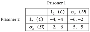(8)

The entries stand for the number of years in prison.

2.1.3. Formal Definition of a Classical Game in the Language of Bits

The formal definition is,

$G_C=\langle N=\left\{\mathrm{1,2}\right\}\mathrm{,}|ij\rangle \mathrm{,}{A}_i=\left\{1_2\mathrm{,}{\sigma }_x\right\}\mathrm{,}{u}_i\mathrm{<mo>\; :\; </mo>}{A}_1\times A_2\to ℝ\rangle \mathrm{<mtext>\; \hspace{0.17em}\; </mtext>\; .}$ (9)

The two differences between this definition and the standard definition of Equation (1) is that the players face an initial two-bit state $|ij\rangle ,i,j=0,1$ presumed by the judge (usually $|00\rangle =\left(C\mathrm{,}C\right)$ and the two-point strategy space of each players contains the two gates $\left(1_2\mathrm{,}{\sigma }_x\right)$ instead of $\left(C\mathrm{,}D\right)$ . The conduction of a pure strategy classical two-players-two strategies simultaneous non-cooperative game given in its normal form (a 2 × 2 payoff matrix) follows the following steps:

1. A referee declares that the initial configuration is some fixed 2 bit state. This initial state is one of the four 2-bit states listed in Equation (4). The referee’s choice does not, in any way, affect the final outcome of the game, it just serves as a starting point. For definiteness assume that the referee suggests the state $|00\rangle$ as the initial state of the game. We already gave an example: In the story of the prisoner dilemma it is like the judge telling them that he assumes that they both confess.

2. In the next step, each player decides upon his strategy ( $1_2$ or ${\sigma }_x$ ) to be applied on his respective bit. For example, if each player chooses the strategy ${\sigma }_x$ we note from Equation (5) that

${\sigma }_x\otimes {\sigma }_x|00\rangle ={\sigma }_x|0\rangle \otimes {\sigma }_x|0\rangle =|1\rangle \otimes |1\rangle =|11\rangle =|DD\rangle .$ (10)

Thus, a player can choose either to leave his bit as suggested by the referee or to change it to the second possible state. As a result of the two operations, the two bit state assumes it final form.

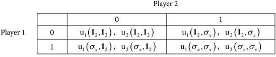
3. The referee then “rewards” each player according to sums appearing in the corresponding payoff matrix. Explicitly,

$\begin{array}{l}{u}_1\left(1_2,1_2\right)=u_2\left(1_2,1_2\right)=-4,u_1\left(1_2,{\sigma }_x\right)=u_2\left({\sigma }_x,1_2\right)=-6,\\ u_1\left({\sigma }_x,1_2\right)=u_2\left(1_2,{\sigma }_x\right)=-2,u_1\left({\sigma }_x,{\sigma }_x\right)=u_2\left({\sigma }_x,{\sigma }_x\right)=-4.\end{array}$

The procedure described above is schematically shown in Figure 1.

A pure strategy Nash equilibrium (PSNE) is a pair of strategies $S_1^{\mathrm{<mo>\; *\; </mo>}}\mathrm{,}{S}_2^{\mathrm{<mo>\; *\; </mo>}}\in {\left\{1_2\mathrm{,}{\sigma }_x\right\}}^2$ such that

$\begin{array}{l}{u}_1\left(S_1\mathrm{,}{S}_2^{\mathrm{<mo>\; *\; </mo>}}\right)\le u_1\left(S_1^{\mathrm{<mo>\; *\; </mo>}}\mathrm{,}{S}_2^{\mathrm{<mo>\; *\; </mo>}}\right)\forall S_1\ne S_1^{\mathrm{<mo>\; *\; </mo>}}\\ u_2\left(S_1^{\mathrm{<mo>\; *\; </mo>}}\mathrm{,}{S}_2\right)\le u_2\left(S_1^{\mathrm{<mo>\; *\; </mo>}}\mathrm{,}{S}_2^{\mathrm{<mo>\; *\; </mo>}}\right)\forall S_2\ne S_2^{\mathrm{<mo>\; *\; </mo>}}\mathrm{.}\end{array}$ (11)

In the present example, it is easy to check that, given the initial state $|00\rangle$ from the referee, the pair of strategies leading to NE is $\left(S_1^{\mathrm{<mo>\; *\; </mo>}}\mathrm{,}{S}_2^{\mathrm{<mo>\; *\; </mo>}}\right)={\sigma }_x\otimes {\sigma }_x$ . However, this equilibrium is not Pareto efficient, namely there is a strategy set $S_1\mathrm{,}{S}_2$ such that $u_i\left(S_1\mathrm{,}{S}_2\right)\ge u\left(S_1^{\mathrm{<mo>\; *\; </mo>}}\mathrm{,}{S}_2^{\mathrm{<mo>\; *\; </mo>}}\right)$ for $i=1,2$ . In the present example the strategy set $1_2\otimes 1_2$ leaves the system in the state $|00\rangle$ and $u_i\left(1_2\mathrm{,}{1}_2\right)=-4>u_i\left({\sigma }_x,{\sigma }_x\right)=-5$ .

Figure 1. A general protocol for a two players two strategies classical game showing the flow of information. To be followed on the figure from left to right. Here $S_1=1_2,{\sigma }_x$ and similarly $S_2=1_2,{\sigma }_x$ . There are only four possible finite states of the system.

2.1.4. Mixed Strategy in the Language of Bits

This technique of operation on bits is naturally extended to treat, mixed strategy games. Then by operating on the bit state $\left(\begin{array}{c}1\\ 0\end{array}\right)$ by the matrix $p{1}_2+\left(1-p\right){\sigma }_x$ with $p\in \left[\mathrm{0,1}\right]$ , we get the vector,

$\left[p\left(\begin{array}{cc}1& 0\\ 0& 1\end{array}\right)+\left(1-p\right)\left(\begin{array}{cc}0& 1\\ 1& 0\end{array}\right)\right]\left(\begin{array}{c}1\\ 0\end{array}\right)=\left(\begin{array}{c}p\\ 1-p\end{array}\right)\mathrm{,}$ (12)

that can be interpreted as a mixed strategy of choosing pure strategy $|1\rangle$ with probability p and pure strategy $|0\rangle$ with probability $1-p$ . Following our example, assuming player 1 chooses $1_2$ with probability p and ${\sigma }_x$ with probability $1-p$ and player 2 chooses $1_2$ with probability q and ${\sigma }_x$ with probability $1-q$ the combined operation on the initial state $|00\rangle$ is,

$\begin{array}{l}\left[p1+\left(1-p\right){\sigma }_x\right]\otimes \left[q1+\left(1-q\right){\sigma }_x\right]|00\rangle \\ =pq|00\rangle +p\left(1-q\right)|01\rangle +\left(1-p\right)q|10\rangle +\left(1-p\right)\left(1-q\right)|11\rangle \end{array}$

3. The Quantum Structure: Qubits

In quantum mechanics, the analog of a bit is a quantum bit, briefly referred to as qubit. Physically, this is a two level system. The simplest example is the two spin states of an electron. In order to explain this concept we need to carry out some preparatory work. For understanding this section, the reader is assumed to be familiar with basic Quantum Mechanics.

3.1. Qubits

The quantum bit (shortly qubit) is the basic unit of quantum information, in the same token that bit is the basic unit of classical information. While the notion of bit is familiar to anyone who has a basic knowledge in information storage (on a hard disk for example) and information transfer, the notion of qubit is much less familiar. Until a few years ago it could be argued that qubit are simple quantum system that cannot be used in such discipline as information science, economics, computational resources and cryptography. This is definitely not the case nowadays as the fields of quantum information and quantum computation become closer and closer to reality. For economists, in general, and for game theorists in particular, the concept of qubit requires some change of mind in the sense that a decision (a strategy) is not simple yes or no (for pure strategy) or simple yes with probability p and no with probability $\left(1-p\right)$ . Similar to the classical game, where a decision is an operation on bits (see Equation (6) a strategy is an operation on qubit. However, since a qubit has a much richer structure than a bit, a quantum strategy is much richer than a classical one. But before speaking of quantum games and quantum strategy we need to define the basic unit (like the hydrogen atom in chemistry).

3.2. Definition and Manipulation of Qubits

A qubit is a vector $|\psi \rangle =a|0\rangle +b|1\rangle \mathrm{,}a\mathrm{,}b\in ℂ$ such that ${\left|a\right|}^2+{\left|b\right|}^2=1$ . The collection $\Sigma \equiv \left\{|\psi \rangle \right\}$ of all qubits is a set and not a space (the vector sum of two qubits is, in general, not a qubit, and hence it has no meaning in what follows). The cardinality of the set of qubits is $\aleph$ (recall that there are only two bits). Two qubits $|\psi \rangle$ and ${\text{e}}^{i\varphi }|\psi \rangle \mathrm{,}\varphi \in ℝ$ that differ by a uni-modular factor ${\text{e}}^{i\varphi }$ are considered identical. This is referred to as phase freedom. A convenient way to underline the difference between bits and qubits is to write them as vectors,

$\text{bit}\text{state}0=\left(\begin{array}{c}1\\ 0\end{array}\right)\mathrm{,}\text{bit}\text{state}1=\left(\begin{array}{c}0\\ 1\end{array}\right)\mathrm{,}\text{qubit}=a\left(\begin{array}{c}1\\ 0\end{array}\right)+b\left(\begin{array}{c}0\\ 1\end{array}\right)=\left(\begin{array}{c}a\\ b\end{array}\right)\mathrm{,}{\left|a\right|}^2+{\left|b\right|}^2=\mathrm{1\; <mtext>\; \hspace{0.17em}\; </mtext>\; .}$ (13)

The definitions used below to denote a qubit are equivalent,

$|\psi \rangle =a|0\rangle +b|1\rangle =a|\uparrow \rangle +b|\downarrow \rangle :=a\left(\begin{array}{c}1\\ 0\end{array}\right)+b\left(\begin{array}{c}0\\ 1\end{array}\right):=\left(\begin{array}{c}a\\ b\end{array}\right),{\left|a\right|}^2+{\left|b\right|}^2=\mathrm{1\; <mtext>\; \hspace{0.17em}\; </mtext>},$ (14)

where $:=$ means, literally, can also be written as. The number of degrees of freedom (parameters) of a qubit is 2 (two complex numbers with one constraint combined with the phase freedom). The phase freedom allows us to chose a to be real and positive. An elegant way to represent a qubit is by choosing two angles $\theta$ and $\varphi$ such that $a=\cos \left(\theta /2\right)$ , $b={\text{e}}^{i\varphi }\sin \left(\theta /2\right)$ , $0\le \theta \le \pi$ , $0\le \varphi \le 2\pi$ :

$\left(\begin{array}{c}a\\ b\end{array}\right)=\left[\cos \left(\theta /2\right)|\uparrow \rangle +{\text{e}}^{i\varphi }\sin \left(\theta /2\right)|\downarrow \rangle \right]=\left(\begin{array}{c}\cos \left(\theta /2\right)\\ {\text{e}}^{i\varphi }\sin \left(\theta /2\right)\end{array}\right)$ (15)

The two angles $\theta$ and $\varphi$ determine a point on the unit sphere (globe) with Cartesian coordinates,

$x=\sin \theta \cos \varphi ,y=\sin \theta \sin \varphi ,z=\cos \theta ,x^2+y^2+z^2=\mathrm{1\; <mtext>\; \hspace{0.17em}\; </mtext>\; .}$ (16)

Therefore, every point on the unit sphere with spherical angles $\left(\theta \mathrm{,}\varphi \right)$ uniquely define a qubit $\left(\begin{array}{c}a\\ b\end{array}\right)$ according to Equation (15). In physics this construction is referred to as Bloch Sphere, as displayed in Figure 2. In particular, the north pole $\theta =0$ corresponds to $|0\rangle =|\uparrow \rangle =\left(\begin{array}{c}1\\ 0\end{array}\right)$ and the south pole, $\theta =\pi$ corresponds to $|1\rangle =|\downarrow \rangle =\left(\begin{array}{c}0\\ 1\end{array}\right)$ .

Figure 2. A qubit $|\psi \rangle$ is represented as a point (a tip of an arrow) on the Bloch sphere.

3.3. Operations on a Single Qubit: Quantum Strategies

In Equations (6) and (7) we defined two classical strategies, $1$ and ${\sigma }_x$ as operations on bits. According to Equation (5) they are realized by 2 × 2 matrices $1=\left(\begin{array}{cc}1& 0\\ 0& 1\end{array}\right)$ , ${\sigma }_x=\left(\begin{array}{cc}0& 1\\ 1& 0\end{array}\right)$ and act on the bit vectors $|0\rangle =\left(\begin{array}{c}1\\ 0\end{array}\right)$ and $|1\rangle =\left(\begin{array}{c}0\\ 1\end{array}\right)$ . In this subsection we develop the quantum analogs: We are interested in operations on qubits, (also referred to as single qubit quantum gates) that transform a qubit $|\psi \rangle =a|0\rangle +b|1\rangle$ into another qubit $a^{\prime }|0\rangle +b^{\prime }|1\rangle$ .

Operations on a single qubit are realized by 2 × 2 complex matrices. We have seen in Figure 2 that a qubit can be represented as a point on the Bloch sphere and therefore, the new qubit must have the same unit length (the radius of the Bloch sphere). In other words the unit length of a qubit must be conserved under any operation. This means that any allowed operation on a qubit is defined by a unitary 2 × 2 matrix U. In the notation of Equation (13) a unitary operation on a qubit represented as a two component vector $\left(\begin{array}{c}a\\ b\end{array}\right)$ is defined as,

$U\left(\begin{array}{c}a\\ b\end{array}\right)=\left(\begin{array}{c}{U}_{11}a+U_{12}b\\ U_{21}a+U_{22}b\end{array}\right)\equiv \left(\begin{array}{c}{a}^{\prime }\\ b^{\prime }\end{array}\right),{\left|a\right|}^2+{\left|b\right|}^2={\left|a^{\prime }\right|}^2+{\left|b^{\prime }\right|}^2=1.$ (17)

For reasons to become clear later on we will restrict ourselves to unitary transformations U with unit determinant, Det[U] = 1. The collection of all 2 × 2 unitary matrices with unit determinant, form a group under the usual rule of matrix multiplication. This is the $SU\left(2\right)$ group that plays a central role in physics. The most general form of a matrix $U\in SU\left(2\right)$ is,

$U\left(\varphi ,\alpha ,\theta \right)=\left(\begin{array}{cc}{\text{e}}^{i\varphi }\cos \frac{\theta }{2}& {\text{e}}^{i\alpha }\sin \frac{\theta }{2}\\ -{\text{e}}^{-i\alpha }\sin \frac{\theta }{2}& {\text{e}}^{-i\varphi }\cos \frac{\theta }{2}\end{array}\right)\mathrm{<mtext>\; \hspace{0.17em}\; </mtext>},0\le \varphi ,\alpha \le 2\pi ,0\le \theta \le \pi \mathrm{<mtext>\; \hspace{0.17em}\; </mtext>\; .}$ (18)

Although we have not yet defined the notion of quantum game, we assert that, in analogy with Equation (6) (that defines player’s classical strategies as operations on bits), the operation on qubits (such that each player acts with his 2 × 2 matrix on his qubit), is an implementation of each player’s quantum strategy. Thus,

Definition In quantum game G_Q based on a classical game G_C with two players and two strategies, the (infinite number of) quantum strategies of each player $i=1,2$ is the infinite set (cardinality $\aleph$ ) of his 2 × 2 matrices $U\left({\varphi }_i\mathrm{,}{\alpha }_i\mathrm{,}{\theta }_i\right)$ as defined in Equation (18).

Since the functional form of the matrix $U\left(\varphi \mathrm{,}\alpha \mathrm{,}\theta \right)$ is given by Equation (18), the strategy of player i is determined by his choice of the three angles ${\gamma }_i=\left({\varphi }_i\mathrm{,}{\alpha }_i\mathrm{,}{\theta }_i\right)$ . The three angles $\varphi \mathrm{,}\alpha \mathrm{,}\theta$ are referred to as the Euler angles. The quantum strategy specified by the 2 × 2 matrix $U\left(\varphi \mathrm{,}\alpha \mathrm{,}\theta \right)$ as specified above has a geometrical interpretation. This is similar to the geometrical interpretation given to qubit as a point on the Bloch sphere in Figure 1, where the two angles $\left(\varphi \mathrm{,}\theta \right)$ determine a point on the boundary of a sphere of unit radius in three dimensions. Such a (Bloch) sphere, is a two dimensional surface denoted by S². On the other hand, the three angles $\varphi \mathrm{,}\alpha \mathrm{,}\theta$ defining a quantum strategy determine a point on the surface of the unit sphere in four dimensional space, ${ℝ}^4$ (the 4 dimensional Euclidean space). The unit sphere is in this space is defined as the collection of points with Cartesian coordinates $\left(x\mathrm{,}y\mathrm{,}z\mathrm{,}w\right)$ restricted by the equation $x^2+y^2+z^2+w^2=1$ . This equality defines the surface of a three dimensional sphere denoted by S³ (impossible to draw a figure). The equality is satisfied by writing the four Cartesian coordinates as,

$x=\sin \theta \sin \varphi \cos \alpha ,y=\sin \theta \sin \varphi ,\sin \alpha ,z=\sin \theta \cos \varphi ,w=\cos \theta \mathrm{<mtext>\; \hspace{0.17em}\; </mtext>\; .}$ (19)

An alternative definition of a player’s strategy is therefore as follows:

Definition A strategy of player i in a quantum analog of a two-players two-strategies classical game is a point ${\gamma }_i=\left({\varphi }_i\mathrm{,}{\alpha }_i\mathrm{,}{\theta }_i\right)\in S^3$ . Thus, instead of a single number 0 or 1 as a strategy of the classical game, the set of quantum strategies has a cardinality ${\aleph }^3=\aleph$ .

Classical Strategies as Special Cases of Quantum Strategies

A desirable property from a quantum game is that the players can reach also their classical strategies. Of course, the interesting case is that reaching the classical strategies does not lead to Nash equilibrium, but the payoff awarded to players in a quantum game that use their classical strategies serve as a useful reference point.

By an appropriate choice of the three angles $\left(\varphi \mathrm{,}\alpha \mathrm{,}\theta \right)$ the quantum strategy $U\left(\varphi \mathrm{,}\alpha \mathrm{,}\theta \right)$ is reduced to one of the two classical strategies $1$ or ${\sigma }_x$ :

$U\left(0,0,0\right)=1=\left(\begin{array}{cc}1& 0\\ 0& 1\end{array}\right),U\left(0,\pi ,\pi \right)={\sigma }_x=\left(\begin{array}{cc}0& 1\\ 1& 0\end{array}\right).$ (20)

3.4. Two Qubit States

In Equations (3) and (4) we represented two-bit states as tensor products of two one-bit states. Equivalently, a two-bit state is represented by a four dimensional vector, three of whose components are 0 and one component is 1 see Equation (3). Since each bit can be found in one of two states $|0\rangle$ or $|1\rangle$ there are exactly four two-bit states. With two-qubit states, the situation is dramatically different in two respects. First, as noted in connection with Equation (14), each qubit $a|0\rangle +b|1\rangle$ with ${\left|a\right|}^2+{\left|b\right|}^2=1$ can be found in an infinite number of states. This is easily understood by noting that, according to Equation (15) and Figure 2, each qubit is a point on the two-dimensional (Bloch) sphere. Accordingly, once we construct two-qubit states by tensor products of two one-qubit states we expect a two-qubit state to be represented by a four dimensional vector of complex numbers. Second, and much more profound, there are four dimensional vectors that are not represented as a tensor product of two two-dimensional vectors. Namely, in contrast with the classical two-bit states, there are two-qubit states that are not represented as a tensor product of two one-qubit states. This is referred to as entanglement and will be explained further below. In a two-players two-strategies classical game, each player has its own bit upon which he can operate (namely, chose his strategy). Below we shall define a quantum game that is based on two-player two-strategies classical game. In such game, each player has its own qubit upon which he can operate by an $SU\left(2\right)$ matrix $U\left(\varphi \mathrm{,}\alpha \mathrm{,}\theta \right)$ (namely, chose his quantum strategy).

Outer (Tensor) Product of Two Qubits

In analogy with Equation (3) that defines the 4 two-bit states we define an outer (or tensor) product of two qubits $|{\psi }_1\rangle \otimes |{\psi }_2\rangle$ using the notation of Equation (13) as follows: Let $|{\psi }_1\rangle =a_1|0\rangle +b_1|1\rangle$ and $|{\psi }_2\rangle =a_2|0\rangle +b_2|1\rangle$ be two qubits numbered 1 and 2. We define their outer (or tensor) product as,

$\begin{array}{c}|{\psi }_1\rangle \otimes |{\psi }_2\rangle =\left(a_1|0\rangle +b_1|1\rangle \right)\otimes \left(a_2|0\rangle +b_2|1\rangle \right)\\ =a_1{a}_2|0\rangle \otimes |0\rangle +a_1{b}_2|0\rangle \otimes |1\rangle +b_1{a}_2|1\rangle \otimes |0\rangle +b_1{b}_2|1\rangle \otimes |1\rangle \mathrm{<mtext>\; \hspace{0.17em}\; </mtext>\; .}\end{array}$ (21)

In terms of 4 component vectors, the tensor products of the elements such as $|0\rangle \otimes |0\rangle$ are the same as the two-bit states defined in Equation (3), and therefore, in this notation we have,

$|{\psi }_1\rangle \otimes |{\psi }_2\rangle =a_1{a}_2\left(\begin{array}{c}1\\ 0\\ 0\\ 0\end{array}\right)+a_1{b}_2\left(\begin{array}{c}0\\ 1\\ 0\\ 0\end{array}\right)+b_1{a}_2\left(\begin{array}{c}0\\ 0\\ 1\\ 0\end{array}\right)+b_1{b}_2\left(\begin{array}{c}0\\ 0\\ 0\\ 1\end{array}\right)=\left(\begin{array}{c}{a}_1{a}_2\\ a_1{b}_2\\ b_1{a}_2\\ b_1{b}_2\end{array}\right)\mathrm{<mtext>\; \hspace{0.17em}\; </mtext>\; .}$ (22)

A tensor product of two qubits as defined above is an example of a two qubit state, briefly referred to as 2qubits. The coefficients of the four products in Equation (21) (or, equivalently, the four vectors in Equation (22)), are complex numbers referred to as amplitudes. Thus, we say that the amplitude of $|0\rangle \otimes |0\rangle$ in the 2 qubits $|{\psi }_1\rangle \otimes |{\psi }_2\rangle$ is $a_1{a}_2$ and so on. Using simple trigonometric identities it is easily verified that the sum of the coefficients is 1, namely,

${\left|a_1{a}_2\right|}^2+{\left|a_1{b}_2\right|}^2+{\left|b_1{a}_2\right|}^2+{\left|b_1{b}_2\right|}^2=\mathrm{1\; <mtext>\; \hspace{0.17em}\; </mtext>\; .}$ (23)

2qubits can also be related to a Bloch sphere S⁵.

We have seen in Equation (22) that a tensor product of two qubits is a 2qubits that is written as a linear combination of the four basic 2qubit states

$|0\rangle \otimes |0\rangle \equiv |00\rangle \mathrm{,}|0\rangle \otimes |1\rangle \equiv |01\rangle \mathrm{,}|1\rangle \otimes |0\rangle \equiv |10\rangle \mathrm{,}|1\rangle \otimes |1\rangle \equiv |11\rangle \mathrm{,}$ (24)

This brings us to the following:

Definition: A general 2qubits $|\Psi \rangle$ has the form,

$\begin{array}{c}|\Psi \rangle =a|0\rangle \otimes |0\rangle +b|0\rangle \otimes |1\rangle +c|1\rangle \otimes |0\rangle +d|1\rangle \otimes |1\rangle \\ =a|00\rangle +b|01\rangle +c|10\rangle +d|11\rangle ,\text{with}{\left|a\right|}^2+{\left|b\right|}^2+{\left|c\right|}^2+{\left|d\right|}^2=1.\end{array}$ (25)

Note the difference between this expression and the outer product of two qubits as defined in Equation (21), in which the coefficients are certain products of the coefficients of the qubit factors. In the expression (25) the coefficients are arbitrary as long as they satisfy the normalization condition. Therefore, Equation (21) is a special case of (25) but not vice-versa. This observation leads us naturally to the next topic, that is, entanglement.

3.5. Entanglement

Entanglement is one of the most fundamental concepts in quantum information and in quantum game theory. In order to introduce it we ask the following question: Let

$|\Psi \rangle =a|00\rangle +b|01\rangle +c|10\rangle +d|11\rangle \mathrm{,}\text{with}{\left|a\right|}^2+{\left|b\right|}^2+{\left|c\right|}^2+{\left|d\right|}^2=\mathrm{1,}$ (26)

[as already defined in Equation (25)], denote a general 2qubits. Is it always possible to represent it as a tensor product of two single qubit states as in Equations (21) or (22)? The answer is NO. Few counter examples with two out of the four coefficients set equal to 0 are,

$|T\rangle \equiv \frac{1}{\sqrt{2}}\left(|01\rangle +|10\rangle \right),|S\rangle \equiv \frac{1}{\sqrt{2}}\left(|01\rangle -|10\rangle \right),|{\psi }_{\pm }\rangle \equiv \frac{1}{\sqrt{2}}\left(|00\rangle \pm i|11\rangle \right)\mathrm{<mtext>\; \hspace{0.17em}\; </mtext>\; .}$ (27)

where the notations T = triplet and S = singlet are borrowed from physics. These four 2qubits are referred to as maximally entangle Bell states. We now have,

Definition A 2qubits state $|\Psi \rangle$ as defined in Equation (26) is said to be entangled iff it cannot be represented as a tensor product of two single qubit states as in Equations (21) or (22).

Entanglement is a pure quantum mechanical concept. It does not occur in manipulations of bits. Thus, there are only four 2bit states as defined in Equation (3), all of them are obtained as tensor products of single bit states, so that by definition they are not entangled. The concept of entanglement is of utmost importance in many aspects of quantum mechanics. It led to a long debate initiated by a paper written in 1935 by Albert Einstein, Boris Podolsky and Nathan Rosen referred to as the EPR paradox that questioned the completeness of quantum mechanics. The answer to this paradox was given by John Bell in 1964. Entanglement plays a central role in quantum information. Here we will see that it also plays a central role in quantum game theory. Strictly speaking, without entanglement, quantum game theory reduces to the classical one.

3.6. Operations on 2qubits (2qubits Gates)

An important tool in manipulating 2qubits is operations transforming one 2qubits to another. Borrowing from the theory of quantum information these are called two-qubit gates. Writing a general 2qubits as defined in Equation (26) in terms of its 4 vector of coefficients,

$|\Psi \rangle =a|00\rangle +b|01\rangle +c|10\rangle +d|11\rangle =\left(\begin{array}{c}a\\ b\\ c\\ d\end{array}\right)\mathrm{<mtext>\; \hspace{0.17em}\; </mtext>},$ (28)

a 2-qubit gate is a unitary 4 × 4 matrix (with unit determinant) acting on the 4 vector of coefficients, in analogy with Equation (17),

$\mathcal{U}\left(\begin{array}{c}a\\ b\\ c\\ d\end{array}\right)=\left(\begin{array}{c}{a}^{\prime }\\ b^{\prime }\\ c^{\prime }\\ d^{\prime }\end{array}\right)\mathrm{<mtext>\; \hspace{0.17em}\; </mtext>},\mathcal{U}\in SU\left(4\right),{\left|a\right|}^2+{\left|b\right|}^2+{\left|c\right|}^2+{\left|d\right|}^2={\left|a^{\prime }\right|}^2+{\left|b^{\prime }\right|}^2+{\left|c^{\prime }\right|}^2+{\left|d^{\prime }\right|}^2=\mathrm{1\; <mtext>\; \hspace{0.17em}\; </mtext>\; .}$ (29)

In the same token as we required the matrices U operating on a single qubit state to have unit determinant, that is, $U\in SU\left(2\right)$ , we require $\mathcal{U}$ also to have a unit determinant, that is, $\mathcal{U}\in SU\left(4\right)$ , the group of 4 × 4 unitary complex matrices with unit determinant.

3.6.1. 2-Qubit Gates Defined as Outer Product of Two 1-Qubit Gates

Let us recall that the two-player strategies in a classical game are defined as outer product of each single player strategy ( $1$ or ${\sigma }_x$ ), defined in Equation (7) that operate on two bit states as exemplified in Equation (10). Let us also recall that each player in a quantum game has a strategy $U\left({\varphi }_i\mathrm{,}{\alpha }_i\mathrm{,}{\theta }_i\right)$ that is a 2 × 2 matrix as defined in Equation (18). Therefore, we anticipate that the two-player strategies in a quantum game are defined as outer product of the two single player strategies. Thus, a 2-qubit gate of special importance is the outer product operation $U=U_1\otimes U_2$ where each player acts on his own qubit. Explicitly, the operation of $\mathcal{U}=U_1\otimes U_2$ on $|\Psi \rangle$ given in (28) is,

$\begin{array}{c}\mathcal{U}|\Psi \rangle \\ =a\left[U_1|0\rangle \right]\otimes \left[U_2|0\rangle \right]+b\left[U_1|0\rangle \right]\otimes \left[U_2|1\rangle \right]\\ +c\left[U_1|1\rangle \right]\otimes \left[U_2|0\rangle \right]+d\left[U_1|1\rangle \right]\otimes \left[U_2|1\rangle \right]\mathrm{<mtext>\; \hspace{0.17em}\; </mtext>\; .}\end{array}$ (30)

Again, before defining the notion of quantum game, we assert that this operation defines the set of combined quantum strategies in analogy with the classical game set of combined strategies defined in Equation (7). Thus, The (infinite numbers of) elements in the set $A_1\times A_2$ of combined (quantum) strategies are 4 × 4 matrices, $U\left({\varphi }_1\mathrm{,}{\alpha }_1\mathrm{,}{\theta }_1\right)\otimes U\left({\varphi }_2\mathrm{,}{\alpha }_2\mathrm{,}{\theta }_2\right)$ . These 4 × 4 matrices act on two qubit states defined above, e.g. Equation (28). The single qubit operations are defined in Equation (17).

3.6.2. Entanglement Operators (Entanglers)

We have already underlined the crucial importance of the concept of entanglement in quantum games. Therefore, of crucial importance for quantum game is an operation executed by an entanglement operator J that acts on a non-entangled 2 qubits and turns it into an entangled 2qubits. Anticipating the importance and relevance of Bell’s states introduced in Equation (27) for quantum games, we search entanglement operators J that operate on the non-entangled state $|0\rangle \otimes |0\rangle =|00\rangle$ and create the maximally entangled Bell states such as $|{\psi }_{+}\rangle$ or $|T\rangle$ as defined in Equation (27). For reason that will become clear later we should require that J is unitary, that is, $J^{†}J=J{J}^{†}=1_4$ . With a little effort we find,

$J_1|00\rangle =\frac{1}{\sqrt{2}}\left(\begin{array}{cccc}1& 0& 0& i\\ 0& 1& -i& 0\\ 0& -i& 1& 0\\ i& 0& 0& 1\end{array}\right)\left(\begin{array}{c}1\\ 0\\ 0\\ 0\end{array}\right)=\frac{1}{\sqrt{2}}\left(\begin{array}{c}1\\ 0\\ 0\\ i\end{array}\right)=\frac{1}{\sqrt{2}}\left(|00\rangle +i|11\rangle \right)=|{\psi }_{+}\rangle \mathrm{<mtext>\; \hspace{0.17em}\; </mtext>\; .}$ (31)

$J_2|00\rangle =\frac{1}{\sqrt{2}}\left(\begin{array}{cccc}0& 1& 0& 1\\ 1& 0& 1& 0\\ 1& 0& 1& 0\\ 0& 1& 0& 1\end{array}\right)\left(\begin{array}{c}1\\ 0\\ 0\\ 0\end{array}\right)=\frac{1}{\sqrt{2}}\left(\begin{array}{c}0\\ 1\\ 1\\ 0\end{array}\right)=\frac{1}{\sqrt{2}}\left(|01\rangle +|10\rangle \right)=|T\rangle \mathrm{<mtext>\; \hspace{0.17em}\; </mtext>\; .}$ (32)

It is straight forward to check that J₁ and J₂ as defined above are unitary and that application of $J_1^{†}$ instead of J₁ on the initial state $|00\rangle$ in Equation (31) yields the second Bell’s state $|{\psi }_{-}\rangle$ also defined in Equation (27), while $J_2^{†}|00\rangle =|S\rangle$ . There is, however, some subtle difference between J₁ and J₂ that will surface later on.

3.6.3. Partial Entanglement Operators

Intuitively, the Bell’s states defined in Equation (27) are Maximally entangled because the two coefficients before the two bit states (say, $|00\rangle$ and $|11\rangle$ ) have the same absolute value, $1/\sqrt{2}$ . We may think of an entangled state where the weights of the two 2-bit states are unequal, in that case we speak of partially entangled state. Thus, instead of the maximally entangled Bell states $|{\psi }_{+}\rangle$ and $|T\rangle$ defined in Equations (27), (31) and (32) we may consider the partially entangled state $|{\psi }_{+}\left(\gamma \right)\rangle$ and $|T\left(\gamma \right)\rangle$ that depend on a continuous parameter (an angle) $0\le \gamma \le \pi$ defined as,

$\begin{array}{l}|{\psi }_{+}\left(\gamma \right)\rangle =\cos \frac{\gamma }{2}|00\rangle +\sin \frac{\gamma }{2}|11\rangle ,\\ |{\psi }_{+}\left(0\right)\rangle =|00\rangle ,|{\psi }_{+}\left(\pi \right)\rangle =|11\rangle ,|{\psi }_{+}\left(\frac{\pi }{2}\right)\rangle =|{\psi }_{+}\rangle \mathrm{<mtext>\; \hspace{0.17em}\; </mtext>\; .}\end{array}$ (33)

$\begin{array}{l}|T\left(\gamma \right)\rangle =\cos \frac{\gamma }{2}|01\rangle +\sin \frac{\gamma }{2}|10\rangle \mathrm{<mtext>\; \hspace{0.17em}\; </mtext>},|T\left(0\right)\rangle =|01\rangle ,\\ |T\left(\pi \right)\rangle =|10\rangle ,|T\left(\frac{\pi }{2}\right)\rangle =|T\rangle \mathrm{<mtext>\; \hspace{0.17em}\; </mtext>\; .}\end{array}$ (34)

The notion of partial entanglement can be put on a more rigorous basis once we have a tool to determine the degree of entanglement. Such a tool does exist, called Entanglement Entropy but it will not be detailed here. The reason for introducing partial entanglement is that it is intimately related with the existence (or the absence) of pure strategy Nash equilibrium in quantum games as will be demonstrated below.

In the same way that we designed the entanglement operators J₁ and J₂ that, upon acting on the two-bit state $|00\rangle$ yield the maximally entangled Bell’s states $|{\psi }_{+}\rangle$ and $|T\rangle$ , we need to design analogous partial entanglement operators $J_{\text{1}}\left(\gamma \right)$ and $J_{\text{2}}\left(\gamma \right)$ that, upon acting on the two-bit state $|00\rangle$ yield the partially entangled states $|{\psi }_{+}\left(\gamma \right)\rangle$ and $|T\left(\gamma \right)\rangle$ . With a little effort we find,

$\begin{array}{l}{J}_1\left(\gamma \right)=\left(\begin{array}{cccc}\cos \frac{\gamma }{2}& 0& 0& i\sin \frac{\gamma }{2}\\ 0& \cos \frac{\gamma }{2}& -i\sin \frac{\gamma }{2}& 0\\ 0& -i\sin \frac{\gamma }{2}& \cos \frac{\gamma }{2}& 0\\ i\sin \frac{\gamma }{2}& 0& 0& \cos \frac{\gamma }{2}\end{array}\right),\\ J_2\left(\gamma \right)=\left(\begin{array}{cccc}0& \cos \frac{\gamma }{2}& 0& -\sin \frac{\gamma }{2}\\ \cos \frac{\gamma }{2}& 0& -\sin \frac{\gamma }{2}& 0\\ \sin \frac{\gamma }{2}& 0& \cos \frac{\gamma }{2}& 0\\ 0& \sin \frac{\gamma }{2}& 0& \cos \frac{\gamma }{2}\end{array}\right)\mathrm{<mtext>\; \hspace{0.17em}\; </mtext>\; .}\end{array}$ (35)

4. Quantum Games

We come now to the main topics of our work, that is, description and search for pure strategy Nash equilibrium in quantum games and the role of entanglement. Quantum games have different structures and different rules than classical games. There are two points that connect a classical game with its quantum analog. First, the quantum game is based on a classical game and the payoffs in the quantum game are determined by the payoff function of the classical game. Second, the classical strategies are obtained as a special case of the quantum strategies. Depending on the entanglement operators J defined in Equation (35), the players may reach the classical square payoffs in the classical game table. In most cases, however, this will not lead to a Nash equilibrium.

4.1. How to Quantize a Classical Game?

With all these complex numbers running around, it must be quite hard to imagine how this formalism can be connected to a game in which people have to take decisions and get tangible rewards that depend on their opponent’s decisions, especially when these rewards are expressed in real numbers (such as dollars or years in prison). To show how it works, we start with a simple classical game (e.g. the prisoner dilemma) and show how to turn into a quantum game that still ends with rewarding its players with tangible rewards. This procedure is referred as quantization of a classical game. We will carry out this task in two steps. In the first step we will consider a classical game and endow each player i with a quantum strategy (The 2 × 2 matrix $U\left({\varphi }_i\mathrm{,}{\alpha }_i\mathrm{,}{\theta }_i\right)$ defined in Eq. (18)). At the same time, we will also design a new payoff system that translates the complex numbers appearing in the state of the system into real numbers in which the reward is given. This first step leads us to a reasonable description of a game, but proves to be inadequate if we want to achieve a really new game, not just the classical game from which we started our journey. This task will be achieved in the second step. In addition, the role of the referee (the judge in the case of the prisoner dilemma) is more significant, as he has to determine the entanglement of the initial state.

Suppose we start with the same classical game as described in section 1, that is given in its normal form with specified payoff functions as,

It is assumed that the referee already decreed that the initial state is $|00\rangle$ , and asks the players to choose their strategies. There is, however, one difference: Instead of using the classical strategies of either leaving a bit untouched (the strategy I) or operating on it with the second strategy ${\sigma }_x$ , the referee allows each player $i=1,2$ to use his quantum strategy $U\left({\varphi }_i\mathrm{,}{\alpha }_i\mathrm{,}{\theta }_i\right)$ defined in Equation (18). Before we find out how all this will help the players, let us find out what will happen with the state of the system after such an operation. For that purpose it is convenient to use the vector notations specified in Equation (2) or (13), (14) and let each player act on his own qubit with his own strategy as explained through Equation (30), thereby leading the system from its initial state $|00\rangle$ to its final state $|\Psi \rangle$ given by,

$\begin{array}{c}|\Psi \rangle =U_1\otimes U_2|00\rangle =U_1|0\rangle \otimes U_2|0\rangle =U_1\left(\begin{array}{c}1\\ 0\end{array}\right)\otimes U_2\left(\begin{array}{c}1\\ 0\end{array}\right)\\ =\left(\begin{array}{c}{\left[U_1\right]}_{11}\\ {\left[U_1\right]}_{21}\end{array}\right)\otimes \left(\begin{array}{c}{\left[U_2\right]}_{11}\\ {\left[U_2\right]}_{21}\end{array}\right)=\left(\begin{array}{c}{\left[U_1\right]}_{11}{\left[U_2\right]}_{11}\\ {\left[U_1\right]}_{11}{\left[U_2\right]}_{21}\\ {\left[U_1\right]}_{21}{\left[U_2\right]}_{11}\\ {\left[U_1\right]}_{21}{\left[U_2\right]}_{21}\end{array}\right)\end{array}$ (36)

With the help of Equation (28) we may then write,

$\begin{array}{c}|\Psi \rangle ={\left[U_1\right]}_{11}{\left[U_2\right]}_{11}|00\rangle +{\left[U_1\right]}_{11}{\left[U_2\right]}_{21}|01\rangle \\ +{\left[U_1\right]}_{21}{\left[U_2\right]}_{11}|10\rangle +{\left[U_1\right]}_{21}{\left[U_2\right]}_{21}|11\rangle \\ \equiv a|00\rangle +b|01\rangle +c|10\rangle +d|11\rangle .\end{array}$ (37)

From Equation (18) it is easy to determine the dependence of the coefficients on the angles (that is the strategies of the two players), for example $a={\left[U_1\right]}_{11}{\left[U_2\right]}_{11}={\text{e}}^{i\left({\varphi }_1+{\varphi }_2\right)}\cos \frac{{\theta }_1}{2}\cos \frac{{\theta }_2}{2}$ and so on. Since $|\Psi \rangle$ is a 2 qubits state, then, as we have stressed all around, in Equations (25) or (29) we have ${\left|a\right|}^2+{\left|b\right|}^2+{\left|c\right|}^2+{\left|d\right|}^2=1$ . This leads us naturally to suggest the following payoff system. The payoff $P_i$ of player i is calculated similar to the calculation of payoffs in correlated equilibrium classical games, with the absolute value squared of the amplitudes $a\mathrm{,}b\mathrm{,}c\mathrm{,}d$ (themselves are complex numbers) as the corresponding probabilities,

$\begin{array}{l}{P}_i\left({\varphi }_1\mathrm{,}{\alpha }_1\mathrm{,}{\theta }_1\mathrm{<mo>\; ;\; </mo>}{\varphi }_2\mathrm{,}{\alpha }_2\mathrm{,}{\theta }_2\right)\\ ={\left|a\right|}^2{u}_i\left(\mathrm{0,0}\right)+{\left|b\right|}^2{u}_i\left(\mathrm{0,1}\right)+{\left|c\right|}^2{u}_i\left(\mathrm{1,0}\right)+{\left|d\right|}^2{u}_i\left(\mathrm{1,1}\right)\mathrm{<mtext>\; \hspace{0.17em}\; </mtext>\; .}\end{array}$ (38)

For example, prisoner’s 1 and 2 years in prison in the prisoner dilemma game table, Equation (8) are,

$P_1=-4{\left|a\right|}^2-6{\left|b\right|}^2-2{\left|c\right|}^2-5{\left|d\right|}^2,P_2=-4{\left|a\right|}^2-2{\left|b\right|}^2-6{\left|c\right|}^2-5{\left|d\right|}^2.$ (39)

The alert reader must have noticed that this procedure ends up in a classical game with mixed strategies. First, once absolute values are taken, the role of the two angles $\varphi$ and $\theta$ is void because

$\begin{array}{l}{\left|a\right|}^2={\cos }^2\frac{{\theta }_1}{2}{\cos }^2\frac{{\theta }_2}{2},{\left|b\right|}^2={\cos }^2\frac{{\theta }_1}{2}{\sin }^2\frac{{\theta }_2}{2},\\ {\left|c\right|}^2={\sin }^2\frac{{\theta }_1}{2}{\cos }^2\frac{{\theta }_2}{2},{\left|d\right|}^2={\sin }^2\frac{{\theta }_1}{2}{\sin }^2\frac{{\theta }_2}{2}.\end{array}$ (40)

What is more disturbing is that we arrive at an old format of classical games with mixed strategies. Since ${\cos }^2\frac{\theta }{2}+{\sin }^2\frac{\theta }{2}=1$ , we immediately identify the payoffs in Equation (38) as those resulting from mixed strategy classical game where a prisoner i chooses to confess with probability ${\cos }^2\frac{{\theta }_i}{2}$ and to don’t confess with probability ${\sin }^2\frac{\theta }{2}$ . In particular, the pure strategies are obtained as specified in Equation (20). Thus while the analysis of the first step taught us how to use quantum strategies and how to design a payoff system applicable for a complex state of the system $|\Psi \rangle$ as defined in Equation (37), it did not prevent us from falling into the trap of triviality in the sense that so far nothing is new.

The reason for this failure is at the heart of quantum mechanics. The initial state $|00\rangle$ upon which the players apply their strategies according to Equation (36) is not entangled; since it is a simple outer product of $|0\rangle$ of player 1 and $|0\rangle$ of player 2, so according to the definition of entanglement given after Equation (27), it is not entangled. Thus we find that: In order for a quantum game to be distinct from its classical analog, the state upon which the two players apply their quantum strategies should be entangled. That is where the entanglement operators J defined in Equations (31), (32) and (35) come into play. Practically, we ask the referee not only to suggest a simple initial state such as $|00\rangle$ but also to choose some entanglement operator J and to apply it on $|00\rangle$ as exemplified in Equations (31), (32) in order to modify it into an entangled state. Only then the players are allowed to apply their quantum strategies, after which the state of the system will be given by $U_1\otimes U_{2}J|00\rangle$ , as compared with Equation (36). There is one more task the referee should take care of. A reasonable desired property is that if, for some reason the players choose to leave everything unchanged by taking ${\gamma }_i=\left({\varphi }_i,{\alpha }_i,{\theta }_i\right)=\left(0,0,0\right)$ , namely, $U_1=U_2=I$ then the final state should be identical to the initial state. This is easily achieved by asking the referee to apply the operator $J^{-1}=$ $J^{†}$ on the state $U_1\otimes U_{2}J|00\rangle$ (that was obtained after the players applied their strategies on the entangled state $J|00\rangle$ . These modification change things entirely, and turn the quantum game into a new game with complicated strategies, that is, it is much richer than its classical analog.

Let us then organize the game protocol as explained above by presenting a list of well defined steps.

1. The starting point is some classical 2 players-2 strategies classical game given in its normal form (a table with utility functions) and a referee whose duty is to choose an initial two bit state and an entanglement operator J.

2. The referee chooses a simple non-entangled 2qubits initial state, which, for convenience, we fix once for all to be $|{\psi }_I\rangle =|00\rangle$ . As in the classical game protocol, the choice of this state does not affect the game in any form, it is just a starting point.

3. The referee then chooses an entanglement operator J and applies it on $|{\psi }_I\rangle$ to generate an entangled state $|{\psi }_{II}\rangle =J|{\psi }_I\rangle$ as exemplified in Equation (31). This operation is part of the rules of the game, namely, it is not possible for the players to affect this choice in any way.

4. At this point each player i applies his own transformation $U_i=U\left({\varphi }_i\mathrm{,}{\alpha }_i\mathrm{,}{\theta }_i\right)$ on his own qubit. The functional dependence of U on the three angles is displayed in Equation (18). This is the only place where the players have to take a decision. After the players made their decisions the product operation is applied on $|{\psi }_{II}\rangle$ as in Equation (30), resulting the state $|{\psi }_{III}\rangle =U_1\otimes U_2|{\psi }_{II}\rangle$ .

5. The referee then applies the inverse of J (namely $J^{†}$ since J is unitary) and gets the final state

$|\Psi \rangle =\stackrel{\text{referee}}{\stackrel{︷}{J^{†}}}\stackrel{\text{players}}{\stackrel{︷}{U_1\otimes U_2}}\stackrel{\text{referee}}{\stackrel{︷}{J|00\rangle }}=a|00\rangle +b|01\rangle +c|10\rangle +d|11\rangle \mathrm{,}$ (41)

where the complex numbers $a\mathrm{,}b\mathrm{,}c\mathrm{,}d$ with ${\left|a\right|}^2+{\left|b\right|}^2+{\left|c\right|}^2+{\left|d\right|}^2=1$ are functions of the elements of U₁ and U₂ namely, following Equation (18), they are functions of the 6 angles $\left({\varphi }_1\mathrm{,}{\alpha }_1\mathrm{,}{\theta }_1\mathrm{<mo>\; ;\; </mo>}{\varphi }_2\mathrm{,}{\alpha }_2\mathrm{,}{\theta }_2\right)$ .

6. The players are then rewarded according to the prescription given by Equation (38).

The set of operations leading from the initial state $|{\psi }_I\rangle$ to the final state $|\Psi \rangle$ is schematically shown in Figure 3.

Figure 3. A general protocol for a two players two strategies quantum game showing the flow of information. Based on Equation (41) to be followed on the figure from left to right. U₁ is player’s 1 move, U₂ is player’s 2 move, and J is an entanglement gate.

4.2. Formal Definition of a Two-Player Pure Strategy Quantum Game

Based on the prescriptions given in Equation (41), Figure (3) and Equation (38) we can now give a formal definition of a two-players two strategies quantum game that is an extension of a classical two-players two strategies game. Necessary ingredient of a quantum game should include:

1. A quantum system which can be analyzed using the tools of quantum mechanics, for example, a two qubits system.

2. Existence of two players, who are able to manipulate the quantum system and operate on their own qubits.

3. A well define strategy set for each player. More concretely, a set of unitary 2 × 2 matrices with unit determinant $U\in SU\left(2\right)$ .

4. A definition of the pay-off functions or utilities associated with the players strategies. More concretely, we have in mind a classical 2-player two strategies game given in its normal form (a table of payoffs).

Definition Given a classical two-players two pure strategies classical game

$G_C=\langle N=\left\{\mathrm{1,2}\right\}\mathrm{,}|ij\rangle \mathrm{,}{A}_i=\left\{I\mathrm{,}{\sigma }_x\right\}\mathrm{,}{u}_i\mathrm{<mo>\; :\; </mo>}{A}_1\otimes A_2\to ℝ\rangle \mathrm{.}$ (42)

Its quantum (pure strategy) analog is the game,

$G_Q=\langle N=\left\{1,2\right\},|{\psi }_I\rangle ,\left\{{\mathcal{A}}_i\right\},J,u_i,P_i\rangle .$ (43)

Here $N=\left\{\mathrm{1,2}\right\}$ , is the set of (two) players, $|{\psi }_I\rangle$ is the initial state suggested by the referee (usually a simple two-bit state such as $|00\rangle$ as in the classical game), ${\mathcal{A}}_i=U\left({\gamma }_i\right)\equiv U_i$ , is the infinite set quantum pure strategies of player i on his qubit defined by the 2 × 2 matrix Equation (18), J is an entanglement operator defined along Equations (31), (32), (41) and Figure 3, $u_i\left(k\mathrm{,}\mathcal{l}\right)$ with $k,\mathcal{l}=0,1$ are the classical payoff functions of the game G and $P_i\left(U_1\mathrm{,}{U}_2\right)$ are the quantum payoff functions defined in Equation (38) in which the coefficients $a\mathrm{,}b\mathrm{,}c\mathrm{,}d$ are complex numbers (also called amplitudes) that determine the expansion of the final state $|\Psi \rangle$ as a combination of two bit states as in Equation (41).

Comments

1) Since $U_i$ is uniquely determined by the three angles ${\gamma }_i=\left({\varphi }_i\mathrm{,}{\alpha }_i\mathrm{,}{\theta }_i\right)$ through Equation (18) we may also regard ${\gamma }_i$ as the strategy of player i. Thus, unlike the classical game where each player has but two strategies, in the quantum game the set of strategies of each player is determined by three continuous variables. As we have already mentioned, the set of strategies of a player correspond to a point on S³.

2) J is part of the rules of the game (it is not controlled by the players). The main requirement from J is that it is a unitary matrix and that after operating on the initial to bit state (taken to be $|00\rangle$ in our case) the result is an entangled 2 qubits.

3) As we stressed in relation with Equation (41), the amplitudes are functions of the two strategies ${\gamma }_i=\left({\varphi }_i\mathrm{,}{\alpha }_i\mathrm{,}{\theta }_i\right)\mathrm{,}\left(i=\mathrm{1,2}\right)$ that are given analytically once the operations implied in Equation (41) are properly carried out (see below).

4.3. Nash Equilibrium in a Pure Strategy Quantum Game

Definition A pure strategy Nash Equilibrium in a quantum game is a pair of strategies $\left({\gamma }_1^{\mathrm{<mo>\; *\; </mo>}}\mathrm{,}{\gamma }_2^{\mathrm{<mo>\; *\; </mo>}}\right)\in S^3\otimes S^3$ (each represents three angles ${\gamma }_i^{\mathrm{<mo>\; *\; </mo>}}=\left({\varphi }_i^{\mathrm{<mo>\; *\; </mo>}}\mathrm{,}{\alpha }_i^{\mathrm{<mo>\; *\; </mo>}}\mathrm{,}{\theta }_i^{\mathrm{<mo>\; *\; </mo>}}\right)\in S^3$ ), such that

$P_1\left({\gamma }_1\mathrm{,}{\gamma }_2^{\mathrm{<mo>\; *\; </mo>}}\right)\le P_1\left({\gamma }_1^{\mathrm{<mo>\; *\; </mo>}}\mathrm{,}{\gamma }_2^{\mathrm{<mo>\; *\; </mo>}}\right)\forall {\gamma }_1\in S^3\mathrm{,}{P}_2\left({\gamma }_1^{\mathrm{<mo>\; *\; </mo>}}\mathrm{,}{\gamma }_2\right)\le P_2\left({\gamma }_1^{\mathrm{<mo>\; *\; </mo>}}\mathrm{,}{\gamma }_2^{\mathrm{<mo>\; *\; </mo>}}\right)\forall {\gamma }_2\in S^3\mathrm{.}$ (44)

It is immediately realized that the concept of Nash equilibrium and its elucidation in a quantum game is far more difficult than the classical one. If each player’s strategy would have been dependent on a single continuous parameter, then the use of the method of best response functions could be effective, but here each player’s strategy depends on three continuous parameters, and the method of response functions might be inadequate. One of the goals of the present work is to alleviate this problem. Another important point concerns the question of cooperation. In the classical prisoner dilemma game, a player that chooses the don’t-confess strategy ( ${\sigma }_x$ ) forces his opponent to cooperate and choose ${\sigma }_x$ (don’t confess) as well, that leads to a pure strategy Nash equilibrium ( ${\sigma }_x\mathrm{,}{\sigma }_x$ ). On the other hand, in the quantum game, the situation is quite different. By looking at the payoff expressions in Equation (39) we see that prisoner 1 wants to reach the state where ${\left|c\right|}^2=1$ and ${\left|a\right|}^2={\left|b\right|}^2={\left|d\right|}^2=0$ , whereas prisoner 2 wants to reach the state where ${\left|b\right|}^2=1$ and ${\left|a\right|}^2={\left|c\right|}^2={\left|d\right|}^2=0$ . Surprisingly, as we shall see below, there are situations such that for every strategy chosen by prisoner 1, prisoner 2 can find a best response that makes ${\left|b\right|}^2=1$ and ${\left|a\right|}^2={\left|c\right|}^2={\left|d\right|}^2=0$ and vice versa, for every strategy chosen by prisoner 2, prisoner 1 can find a best response that makes ${\left|c\right|}^2=1$ and ${\left|a\right|}^2={\left|b\right|}^2={\left|d\right|}^2=0$ . Since the two situations cannot occur simultaneously, there is no Nash equilibrium and no cooperation in this case.

The Role of the Entanglement Operator J and Classical Commensurability

A desired property (although not crucial) of a quantum game is that the theory as defined in Equation (41) and Figure 3 includes the classical game as a special case. We already know from Equation (20) that the classical strategies I and ${\sigma }_x$ are obtained as special cases of the quantum ones, since $U\left(\mathrm{0,0,0}\right)=I$ and $U\left(\mathrm{0,0,}\pi \right)={\sigma }_x$ . What we require here is that by using their classical strategies, the players will be able to reach the four classical states (squares of the game table). For example, to reach the square (C, C) the coefficients $a\mathrm{,}b\mathrm{,}c\mathrm{,}d$ in the final state $|\Psi \rangle$ at the end of the game (see Equation (41) should be ${\left|a\right|}^2=1,$ $b=c=d=0$ and so on. For this requirement to hold, the entanglement operator J should satisfy a certain equality. We refer to this equality to be satisfied by J as classical commensurability. From the discussion around Equation (20) we recall that in a classical game, the only operations on bits are implemented either

by the unit matrix I (leave the bit in its initial state $|0\rangle$ or $|1\rangle$ ) or ${\sigma }_x=\left(\begin{array}{cc}0& 1\\ 1& 0\end{array}\right)$ (change the state of the bit from $|0\rangle$ to $|1\rangle$ or vice versa). Thus, by choosing $U\left(\mathrm{0,0,0}\right)$ or $U\left(\mathrm{0,0,}\pi \right)$ the players virtually use classical strategies. Therefore, classical commensurability implies

$\left[{\sigma }_x\otimes {\sigma }_x\mathrm{,}J\right]=\mathrm{0,}\left(\text{Classical}\text{commensurability}\right)\mathrm{,}$ (45)

Indeed, if this condition is satisfied and both U₁ and U₂ are classical strategies, then $\left[U_1\otimes U_2\mathrm{,}J\right]=0$ because in this case $U_1\otimes U_2=I\otimes I$ or $I\otimes {\sigma }_x$ or ${\sigma }_x\otimes I$ or ${\sigma }_x\otimes {\sigma }_x$ and as we show below, all of the four operators commute with J. Consequently

$|\Psi \rangle =J^{†}{U}_1\otimes U_{2}J|00\rangle =J^{†}J{U}_1\otimes U_2|00\rangle =U_1\otimes U_2|00\rangle ,$ (46)

that is what happens in a classical game as explained in connection with Figure 1. To prove that the four two-player classical strategies listed above do commute with J we note that by direct calculations it is easy to show that J₁ defined in Equation (31) satisfies classical commensurability because an elementary manipulation of matrices shows that J₁ can be written as

$J_1={\text{e}}^{i\frac{\pi }{4}{\sigma }_x\otimes {\sigma }_x}=\frac{1}{\sqrt{2}}\left(1_4+i{\sigma }_x\otimes {\sigma }_x\right),$ (47)

and this matrix naturally commutes with ${\sigma }_x\otimes {\sigma }_x$ . On the other hand, $J_2$ defined in Equation (32) does not satisfy classical commensurability as can be checked by directly inspecting the commutation relation $\left[{\sigma }_x\otimes {\sigma }_x\mathrm{,}{J}_2\right]\ne 0$ .

4.4. Absence of Nash Equilibrium for Maximally Entangled States

After defining the notion of quantum games and their pure strategy Nash Equilibrium we face the problem of finding pure strategy Nash Equilibrium. The first result in this area is negative: If the state $|{\psi }_I\rangle =J|00\rangle$ is maximally entangled, (e.g., $|{\psi }_I\rangle =|{\psi }^{+}\rangle$ (Equation (31)) or $|{\psi }_I\rangle =|T\rangle$ (Equation (32)) the quantum game of the prisoner dilemma does not have a pure strategy Nash Equilibrium. Our poof of this statement will be straightforward. First we will calculate explicitly the amplitudes $a\mathrm{,}b\mathrm{,}c\mathrm{,}d$ of the final wave function $|\Psi \rangle$ as defined in Equation (41) and in Figure 3 and then use the method of response functions and show that the two response functions $B_2\left({\gamma }_1\right)$ and $B_1\left({\gamma }_2\right)$ cannot intersect.

4.4.1. Calculating the Amplitudes of the Final States $|\Psi \rangle$

In order to calculate the payoffs P₁ and P₂ according to the prescription (39) we need to carry out the operations specified in Equation (41) leading from the initial state $|00\rangle$ all the way to the final state $|\Psi \rangle$ . This is a standard manipulation in matrix multiplication that in the present case ends up with reasonable (not so long) expressions. As an example we consider the entanglement operator $J=J_1$ as given in Equation (31) so that $J|00\rangle =|{\psi }^{+}\rangle$ that is a Maximally Entangled State: Player i has a strategy matrix $U_i\equiv U\left({\gamma }_i\right)=U\left({\varphi }_i\mathrm{,}{\alpha }_i\mathrm{,}{\theta }_i\right)$ as defined in Equation (18). The product $U\left({\gamma }_1\right)\otimes U\left({\gamma }_2\right)$ acts on $|{\psi }_{+}\rangle$ according to the prescription (30) is given explicitly as,

$U_1\otimes U_2|{\psi }_{+}\rangle =\frac{1}{\sqrt{2}}\left[\left(U_1|0\rangle \right)\otimes \left(U_2|0\rangle \right)+i\left(U_1|1\rangle \right)\otimes \left(U_2|1\rangle \right)\right]\mathrm{<mtext>\; \hspace{0.17em}\; </mtext>\; .}$ (48)

Explicitly, for a 2 × 2 matrix $U=\left(\begin{array}{cc}{U}_{11}& U_{12}\\ U_{21}& U_{22}\end{array}\right)$ we have, according to Equation (17),

$\begin{array}{l}U|0\rangle =U\left(\begin{array}{c}1\\ 0\end{array}\right)=\left(\begin{array}{c}{U}_{11}\\ U_{21}\end{array}\right)=U_{11}|0\rangle +U_{21}|1\rangle ,\\ U|1\rangle =U\left(\begin{array}{c}0\\ 1\end{array}\right)=\left(\begin{array}{c}{U}_{12}\\ U_{22}\end{array}\right)=U_{12}|0\rangle +U_{22}|1\rangle \mathrm{<mtext>\; \hspace{0.17em}\; </mtext>\; .}\end{array}$ (49)

Performing the outer products as in Equation (21), multiplying by $J^{†}$ we can find the corresponding amplitudes $a\mathrm{,}b\mathrm{,}c\mathrm{,}d$ of $|\Psi \rangle$ in the notation of (21) or (28). Straight forward but tedious calculations yield,

Coefficients of $|\Psi \rangle$ for $J|00\rangle =|{\psi }_{+}\rangle$ (Equation (31)),

$\begin{array}{l}{\left|a\right|}^2={\left[\cos \frac{1}{2}{\theta }_1\cos \frac{1}{2}{\theta }_2\cos \left({\varphi }_1+{\varphi }_2\right)-\sin \frac{1}{2}{\theta }_1\sin \frac{1}{2}{\theta }_2\sin \left({\alpha }_1+{\alpha }_2\right)\right]}^2\mathrm{,}\\ {\left|b\right|}^2={\left[\cos \frac{1}{2}{\theta }_1\sin \frac{1}{2}{\theta }_2\cos \left({\varphi }_1-{\alpha }_2\right)+\sin \frac{1}{2}{\theta }_1\cos \frac{1}{2}{\theta }_2\sin \left({\alpha }_1-{\varphi }_2\right)\right]}^2\mathrm{,}\\ {\left|c\right|}^2={\left[\sin \frac{1}{2}{\theta }_1\cos \frac{1}{2}{\theta }_2\cos \left({\alpha }_1-{\varphi }_2\right)-\cos \frac{1}{2}{\theta }_1\sin \frac{1}{2}{\theta }_2\sin \left({\varphi }_1-{\alpha }_2\right)\right]}^2\mathrm{,}\\ {\left|d\right|}^2={\left[\cos \frac{1}{2}{\theta }_1\cos \frac{1}{2}{\theta }_2\sin \left({\varphi }_1+{\varphi }_2\right)+\sin \frac{1}{2}{\theta }_1\sin \frac{1}{2}{\theta }_2\cos \left({\alpha }_1+{\alpha }_2\right)\right]}^2\mathrm{<mtext>\; \hspace{0.17em}\; </mtext>\; .}\end{array}$ (50)

Compared with Equation (40) we see that the present game is really novel, all the angles appear in the payoff and it is not reducible to any form of classical game.

It is instructive to check how the classical strategies are recovered as special cases of the quantum ones. If both players choose $U\left(\mathrm{0,0,0}\right)=I$ then ${\left|a\right|}^2=1$ and $|\Psi \rangle =|00\rangle$ with amplitude 1, that corresponds to the classical strategy ( $1_2\mathrm{,}{1}_2$ ) leading to the state (C, C). Similarly, if one player chooses $U\left(\mathrm{0,0,0}\right)$ and the other chooses $U\left(\mathrm{0,0,}\pi \right)$ this leads to either ${\left|b\right|}^2=1$ corresponding to classical strategies ( $1_2\mathrm{,}{\sigma }_x$ ) leading to the state (C, D) or to ${\left|c\right|}^2=1$ corresponding to classical strategies ( ${\sigma }_x\mathrm{,}I$ ). leading to the state (D, C). Finally, if both players choose $U\left(\mathrm{0,0,}\pi \right)$ then the final state is $|\Psi \rangle =|11\rangle$ with amplitude 1, that corresponds to the classical strategy ( ${\sigma }_x\mathrm{,}{\sigma }_x$ ) leading to the state (D, D). Unlike the classical game, however, this choice is, in general, not a Nash equilibrium. Player 1 for example may find a strategy $U\left({\varphi }_1\mathrm{,}{\alpha }_1\mathrm{,}{\theta }_1\right)$ such that $P_1\left[U\left({\varphi }_1,{\alpha }_1,{\theta }_1\right),{\sigma }_x\right]>-4$ . The upshot then is that if classical commensurability is respected, then, by using classical strategies the players can reach the classical positions (C, C), (C, D), (D, C) and (D, D) but the classical Nash equilibrium is not relevant for the quantum game.

Example 2: Triplet Bell State: If we take $J=J_2$ as in Equation (32) we get $J|00\rangle =|T\rangle$ , the triplet Bell state. Performing the calculations $|\Psi \rangle =J^{†}{U}_1\otimes U_2|T\rangle$ we get the four probabilities,

Coefficients of $|\Psi \rangle$ for $J|00\rangle =|T\rangle$ = Bell’s Triplet State, (Equation (32))

$\begin{array}{l}{\left|a\right|}^2={\left[\cos \frac{1}{2}{\theta }_1\cos \frac{1}{2}{\theta }_2\cos \left({\varphi }_1-{\varphi }_2\right)-\sin \frac{1}{2}{\theta }_1\sin \frac{1}{2}{\theta }_2\cos \left({\alpha }_1-{\alpha }_2\right)\right]}^2,\\ {\left|b\right|}^2={\left[\cos \frac{1}{2}{\theta }_1\sin \frac{1}{2}{\theta }_2\sin \left({\varphi }_1+{\alpha }_2\right)+\sin \frac{1}{2}{\theta }_1\cos \frac{1}{2}{\theta }_2\sin \left({\alpha }_1+{\varphi }_2\right)\right]}^2,\\ {\left|c\right|}^2={\left[\sin \frac{1}{2}{\theta }_1\sin \frac{1}{2}{\theta }_2\sin \left({\alpha }_1-{\alpha }_2\right)-\cos \frac{1}{2}{\theta }_1\cos \frac{1}{2}{\theta }_2\sin \left({\varphi }_1-{\varphi }_2\right)\right]}^2,\\ {\left|d\right|}^2={\left[\sin \frac{1}{2}{\theta }_1\cos \frac{1}{2}{\theta }_2\cos \left({\alpha }_1+{\varphi }_2\right)+\cos \frac{1}{2}{\theta }_1\sin \frac{1}{2}{\theta }_2\cos \left({\varphi }_1+{\alpha }_2\right)\right]}^2\mathrm{<mtext>\; \hspace{0.17em}\; </mtext>\; .}\end{array}$ (51)

4.4.2. Proof of Absence of Pure strategy Nash Equilibrium

The following theorem is well known, see for example Refs. [16] [17] [28] . Here we prove it directly by showing the best response functions cannot intersect.

Theorem The quantum game defined as in Equation (43) with $J=J_1$ as given by Equation (31) does not have a pure strategy Nash Equilibrium.

Proof From the expressions (50) for the amplitudes it is evident that for any strategy $\left({\alpha }_1\mathrm{,}{\varphi }_1\mathrm{,}{\theta }_1\right)$ of player 1, player 2 can find a best response that brings him to the minimum years in prison with

$B_2\left({\varphi }_1,{\alpha }_1,{\theta }_1\right)=U\left({\varphi }_2={\alpha }_1-\frac{\pi }{2},{\alpha }_2={\varphi }_1,{\theta }_2={\theta }_1\right),$ (52)

because then we have ${\left|b\right|}^2=1,{\left|a\right|}^2={\left|c\right|}^2={\left|d\right|}^2=0$ . Similarly, for any strategy $\left({\alpha }_2\mathrm{,}{\varphi }_2\mathrm{,}{\theta }_2\right)$ of player 2, player 1 can find a best response that brings him to the minimum years in prison with

$B_1\left({\varphi }_2,{\alpha }_2,{\theta }_2\right)=U\left({\varphi }_1={\alpha }_2-\frac{\pi }{2},{\alpha }_1=\frac{\pi }{2}+{\varphi }_2,{\theta }_1=\pi -{\theta }_2\right),$ (53)

because then we have, ${\left|c\right|}^2=1,{\left|a\right|}^2={\left|b\right|}^2={\left|d\right|}^2=0$ Evidently, the two restrictions on the amplitudes cannot occur simultaneously, and therefore, the two response functions cannot intersect. Hence, there is no pure strategy Nash equilibrium. □

Similarly, the quantum game defined as in Equation (43) with $J=J_2$ as given by Equation (32) does not have a pure strategy Nash Equilibrium. Simple manipulations based on expressions (51) for the amplitudes lead to the following response functions,

$B_2\left({\varphi }_1,{\alpha }_1,{\theta }_1\right)=U\left({\varphi }_2={\alpha }_1-\frac{\pi }{2},{\alpha }_2=\frac{\pi }{2}-{\varphi }_1,{\theta }_2=\pi -{\theta }_1\right).$ (54)

$B_1\left({\varphi }_2,{\alpha }_2,{\theta }_2\right)=U\left({\varphi }_1={\varphi }_2-\frac{\pi }{2},{\alpha }_1=\frac{\pi }{2}+{\alpha }_2,{\theta }_1={\theta }_2\right).$ (55)

It is worth emphasizing that these (negative) results are valid only if the classical game upon which the quantum game is built does not have a Pareto efficient pure strategy Nash equilibrium. If such equilibrium exists, the players will choose their quantum strategies to settle on this place. For example, if, in some special prisoner dilemma game there is a Pareto efficient equilibrium in (C, C) then both players prefer $\left|a^2\right|=1,{\left|b\right|}^2={\left|c\right|}^2={\left|d\right|}^2=0$ . For the first game (Equation (50)) they will choose ${\theta }_1={\theta }_2$ , ${\alpha }_1+{\alpha }_2=\pi /2$ , ${\varphi }_1+{\varphi }_2=\pi$ , while for the second game (Equation (51)) they will choose ${\theta }_1={\theta }_2$ , ${\varphi }_1={\varphi }_2$ , ${\alpha }_1-{\alpha }_2=\pi$ .

Starting from a non-entangled initial state (for example $|00\rangle$ and using entanglement operators J as defined in Equations (31) or (32) leading to the maximally entangled states $|{\psi }_{+}\rangle$ and $|T\rangle$ respectively, the quantum game has no pure strategy NE.

The natural place to look for NE is then to consider a mixed strategy. Before that, however, we want to consider the concept of partial entanglement, since, as we shall show, it can lead to a pure strategy Nash equilibrium of the quantum game.

5. Nash Equilibrium with Partial Entanglement

We have seen in subsection 4.4 that when the entanglement operator J appearing in Equation (41) or, alternatively, in Figure 3, leads to a maximally entangled state $|{\psi }_{+}\rangle$ or $|T\rangle$ , the quantum game does not have pure strategy Nash equilibrium. We also know that when $J=1_{4\times 4}$ , then the classical Nash Equilibrium obtains because the state prepared by the referee for the two players to apply their strategies is just the initial state $|00\rangle$ and the players then use their classical strategies as special case of their quantum ones $|{\psi }_{+}\rangle$ . This may lead to the following scenario: Suppose J is classically commensurate, but displays only partial entanglement (explicitly this corresponds to $J\left(\beta \right)=J_1\left(\beta \right)$ given in Equation (56) with $0<\beta <\frac{\pi }{2}$ ). Then there may be a threshold value $0<{\beta }_c<\frac{\pi }{2}$ such that for $0\le \beta <{\beta }_c$ there is a pure strategy Nash Equilibrium (that may coincide or may be distinct from the classical one) while for $\beta >{\beta }_c$ there is no pure strategy Nash Equilibrium because J is close to the case of maximal entanglement. In this section we will check this hypothesis numerically using the method of response functions and show that this scenario is possible and that the quantum Nash equilibrium might be distinct (and ameliorates) the classical one. In the first subsection we will explain the method of response functions, while in the second subsection the numerical algorithm will be explained.

5.1. Partial Entanglement

The states $|{\psi }_{+}\rangle$ and $|T\rangle$ defined in Equations (31) and (32) are “maximally entangled” in the sense that the absolute value square of the two coefficient before the 2-bit states are equal to 1/2 so that the corresponding weights are equal. If the weights are unequal, we have partial entanglement.

Partial Entanglement Operator with Classical Commensurability

We have already pointed out that the entanglement operator J as defined in Equation (31) satisfies classical commensurability $\left[{\sigma }_x\otimes {\sigma }_x\mathrm{,}J\right]=0$ . We now reconsider the operator $J_1\left(\beta \right)$ defined in the first equality of Equation (35). It can be written as

$J_1\left(\beta \right)={\text{e}}^{i\frac{\beta }{2}{\sigma }_x\otimes {\sigma }_x}=\cos \frac{\beta }{2}{I}_{4\times 4}+i\sin \frac{\beta }{2}{\sigma }_x\otimes {\sigma }_x\mathrm{<mtext>\; \hspace{0.17em}\; </mtext>\; .}$ (56)

Clearly, when $\beta =0$ we have $J_1\left(0\right)=I_{4\times 4}$ while $J\left(\frac{\pi }{2}\right)$ is given in Equation (22) that leads to the maximally entangled state $|{\psi }_{+}\rangle$ on the RHS of Equation (31). For $0<\beta <\frac{\pi }{2}$ , $J\left(\beta \right)$ is a partial entanglement operator and the state $J_1\left(\beta \right)|00\rangle =|{\psi }_{+}\left(\beta \right)\rangle$ defined in Equation (33) is said to be partially entangled. When $J_1\left(\beta \right)$ is used in Equation (41) it results in the final state $|\Psi \rangle =a|00\rangle +b|01\rangle +c|10\rangle +d|11\rangle$ with complex amplitudes,

$\begin{array}{l}a=[\cos \frac{1}{2}{\theta }_1\cos \frac{1}{2}{\theta }_2\cos \left({\varphi }_1+{\varphi }_2\right)-\sin \frac{1}{2}{\theta }_1\sin \frac{1}{2}{\theta }_2\sin \left({\alpha }_1+{\alpha }_2\right)\sin \beta \\ +i\cos \frac{1}{2}{\theta }_1\cos \frac{1}{2}{\theta }_2\sin \left({\varphi }_1+{\varphi }_2\right)\cos \beta ],\\ b=[\cos \frac{1}{2}{\theta }_1\sin \frac{1}{2}{\theta }_2\cos \left({\varphi }_1-{\alpha }_2\right)+\sin \frac{1}{2}{\theta }_1\cos \frac{1}{2}{\theta }_2\sin \left({\alpha }_1-{\varphi }_2\right)\sin \beta \\ +i\cos \frac{1}{2}{\theta }_1\sin \frac{1}{2}{\theta }_2\sin \left({\varphi }_1-{\alpha }_2\right)\cos \beta ],\end{array}$

$\begin{array}{l}c=[\sin \frac{1}{2}{\theta }_1\cos \frac{1}{2}{\theta }_2\cos \left({\alpha }_1-{\varphi }_2\right)-\cos \frac{1}{2}{\theta }_1\sin \frac{1}{2}{\theta }_2\sin \left({\varphi }_1-{\alpha }_2\right)\sin \beta \\ -i\sin \frac{1}{2}{\theta }_1\cos \frac{1}{2}{\theta }_2\sin \left({\alpha }_1-{\varphi }_2\right)\cos \beta ],\\ d=[\sin \frac{1}{2}{\theta }_1\sin \frac{1}{2}{\theta }_2\cos \left({\alpha }_1+{\alpha }_2\right)+\cos \frac{1}{2}{\theta }_1\cos \frac{1}{2}{\theta }_2\sin \left({\varphi }_1+{\varphi }_2\right)\sin \beta \\ -i\sin \frac{1}{2}{\theta }_1\sin \frac{1}{2}{\theta }_2\sin \left({\alpha }_1+{\alpha }_2\right)\cos \beta ]\mathrm{.}\end{array}$ (57)

For $\beta =\frac{\pi }{2}$ the squares ${\left|a\right|}^2,{\left|b\right|}^2,{\left|c\right|}^2,{\left|d\right|}^2$ are reduced to their values in Equation (50). We will check below the existence of pure strategy Nash equilibrium for $0<\beta <\frac{\pi }{2}$ .

5.2. Best Response Functions

The method of best response functions is an effective method for locating Nash equilibrium in classical games with two players in which the strategy space is not complicated. Its effectiveness for the quantum game is not at all evident due to the complexity of strategy space that is a surface of the sphere S³. The method that will be used below is to replace continuous variables $\varphi \mathrm{,}\alpha \mathrm{,}\theta$ by a mesh of discrete points. This turns the problem to a one with finite (albeit very large) strategy space for which the method of response functions is expected to work. Therefore, we shall explain the method on the most elementary level as taught in undergraduate courses in game theory.

5.2.1. Finite Set of Strategies

Let us consider a two-player classical game where each player i has K strategies, denoted as $\left\{k_i\right\},i=1,2$ , $k_i=1,2,\cdots ,K$ . For each strategy k₁ of player 1, player 2 finds a best response strategy $q_2\left(k_1\right)$ that leads him to the highest possible payoff once k₁ is given (here q₂ is an integer between 1 and K). (The notation used here for the response functions is $q_i\left(\mathrm{.}\right)$ instead of $B_i\left(\mathrm{.}\right)$ ). Similarly, for each strategy k₂ of player 2, player 1 finds a best response strategy $q_1\left(k_2\right)$ that leads him to the highest possible payoff once k₂ is given. It should be stressed that the mapping $q_1\mathrm{<mo>\; :\; </mo>}\left\{\mathrm{1,2,}\cdots \mathrm{,}K\right\}\to \left\{\mathrm{1,2,}\cdots \mathrm{,}K\right\}$ is not necessarily one-to-one. There may be more than one response to a given strategy and there may be strategies that are not chosen as best response. We can now draw two discrete “curves”. The first curve is obtained by listing k₁ along the x axis and plotting the points $q_2\left(k_1\right)$ above the x axis. The second curve is obtained by listing k₂ along the y axis and plotting the points $q_1\left(k_2\right)$ to the right of the y axis. These discrete curves need not be monotonic, and they may not have a common point. However, if the discrete curves do have a common point $\left(q_1^{\mathrm{<mo>\; *\; </mo>}}\mathrm{,}{q}_2^{\mathrm{<mo>\; *\; </mo>}}\right)$ this pair of strategies forms a Nash equilibrium. The point $\left(q_1^{\mathrm{<mo>\; *\; </mo>}}\mathrm{,}{q}_2^{\mathrm{<mo>\; *\; </mo>}}\right)$ can be found graphically or else, once the lists $q_2\left(k_1\right)$ and $q_1\left(k_2\right)$ are prepared, the equilibrium strategies are found by searching solution to the equation

$\left|q_1^{\mathrm{<mo>\; *\; </mo>}}-q_1\left(q_2^{\mathrm{<mo>\; *\; </mo>}}\right)\right|+\left|q_2^{\mathrm{<mo>\; *\; </mo>}}-q_2\left(q_1^{\mathrm{<mo>\; *\; </mo>}}\right)\right|=\mathrm{0\; <mtext>\; \hspace{0.17em}\; </mtext>\; .}$ (58)

5.2.2. Continuous Set of Strategies

The method of best response functions is also effective when the strategy spaces are determined by single continuous parameters, $x_1\in \left[a_1\mathrm{,}{b}_1\right]$ (for player 1) and $x_2\in \left[a_2\mathrm{,}{b}_2\right]$ (for player 2). The response functions are $q_2\left(x_1\right)$ and $q_1\left(x_2\right)$ where, following the discrete case, $q_1\left(x_2\right)$ need not be one-to-one and need not be a continuous function. Its domain is defined on $x_2\in \left[a_2\mathrm{,}{b}_2\right]$ and its target is defined in $\left[a_1\mathrm{,}{b}_1\right]$ . Analogous statements hold for $q_2\left(x_1\right)$ . The two functions are now plotted as explained above for the discrete case and Nash equilibrium may obtain at strategies $\left(q_1^{\mathrm{<mo>\; *\; </mo>}}\mathrm{,}{q}_2^{\mathrm{<mo>\; *\; </mo>}}\right)\in \left[a_1\mathrm{,}{b}_1\right]\times \left[a_2\mathrm{,}{b}_2\right]$ such that,

$q_1^{*}=q_1\left(q_2^{*}\right),q_2^{*}=q_2\left(q_1^{*}\right)\mathrm{<mtext>\; \hspace{0.17em}\; </mtext>\; .}$ (59)

Unfortunately, this method is ineffective when each strategy space is determined by more than one continuous variable as in our quantum game where the strategy of player $i=1,2$ is determined by three angular variables, $0\le {\varphi }_i\le 2\pi$ , $0\le {\alpha }_i\le 2\pi$ , $0\le {\theta }_i\le \pi$ or, in short notation, ${\gamma }_i=\left({\varphi }_i\mathrm{,}{\alpha }_i\mathrm{,}{\theta }_i\right)$ being a point on S³. The response functions $q_1\left({\gamma }_2\right)$ and $q_2\left({\gamma }_1\right)$ are mappings from S³ to S³. They are not necessarily one-to-one but continuous. However, any attempt to search for Nash equilibrium using the methods as described above for the simple cases is useless.

5.3. Quantum Game with Finite Set of Strategies

Since it is practically useless to follow the procedure of best response functions in the 6 dimensional spaces of pure strategies ${\gamma }_1\otimes {\gamma }_2$ we discretize the continuous variables $\varphi \mathrm{,}\alpha \mathrm{,}\theta$ in a series of steps as follows: [29] .

1. The variable $0\le \theta \le \pi$ will assume $N_{\theta }$ values $\theta \left(1\right)=0<\theta \left(2\right)<\theta \left(3\right)<\cdots <\theta \left(N_{\theta }\right)=\pi$ . They are assumed to be equally spaced, the spacing is then $\frac{\pi }{N_{\theta }-1}$ .

2. For every $\theta \left(k_{\theta }\right)$ with $1<k_{\theta }<N_{\theta }$ the variable $0\le \varphi \le 2\pi$ will assume $N_{\varphi }$ values $\varphi \left(1\right)=0<\varphi \left(2\right)<\theta \left(3\right)<\cdots <\varphi \left(N_{\varphi }\right)=2\pi$ . They are assumed to be equally spaced, the spacing is then $\frac{2\pi }{N_{\varphi }-1}$ . For $\theta \left(1\right)=0$ and for $\theta \left(1\right)=\pi$ the variable $\varphi$ assumes the single value $\varphi \left(1\right)=0$ .

3. For every $\theta \left(k_{\theta }\right)$ with $1<k_{\theta }<N_{\theta }$ the variable $0\le \alpha \le 2\pi$ will assume $N_{\alpha }$ values $\alpha \left(1\right)=0<\alpha \left(2\right)<\theta \left(3\right)<\cdots <\alpha \left(N_{\alpha }\right)=2\pi$ . They are assumed to be equally spaced, the spacing is then $\frac{2\pi }{N_{\alpha }-1}$ . For $\theta \left(1\right)=0$ and for $\theta \left(1\right)=\pi$ the variable $\alpha$ assumes the single value $\alpha \left(1\right)=0$ .

4. The total number of strategies of each player is the $N_S=\left(N_{\theta }-2\right)N_{\varphi }{N}_{\alpha }+2$ .

5. We can now construct a $1\leftrightarrow 1$ lexicographic order among triples $\left(\varphi \left(k_{\varphi }\right)\mathrm{,}\alpha \left(k_{\alpha }\right)\mathrm{,}\theta \left(k_{\theta }\right)\right)$ of angles, corresponds to a single integer $1\le I\left(k_{\varphi }\mathrm{,}{k}_{\alpha }\mathrm{,}{k}_{\theta }\right)\le N_S$ . For example,

$I\left(k_{\varphi },k_{\alpha },k_{\theta }\right)>I\left({k^{\prime }}_{\varphi },{k^{\prime }}_{\alpha },{k^{\prime }}_{\theta }\right)\text{if}(\begin{array}{l}{k}_{\theta }>{k^{\prime }}_{\theta }\text{or}\\ k_{\theta }={k^{\prime }}_{\theta }\text{but}{k}_{\varphi }>{k^{\prime }}_{\varphi }\text{or}\\ k_{\theta }={k^{\prime }}_{\theta }\text{and}{k}_{\varphi }={k^{\prime }}_{\varphi }\text{but}{k}_{\alpha }>{k^{\prime }}_{\alpha }\mathrm{<mtext>\; \hspace{0.17em}\; </mtext>\; .}\end{array}$ (60)

In this way a set of three continuous variables $\left(\varphi \mathrm{,}\alpha \mathrm{,}\theta \right)$ is replaced by a single discrete variable $1\le I\le N_S$ that uniquely determine the $N_S$ triples $\left[\varphi \left(I\right)\mathrm{,}\alpha \left(I\right)\mathrm{,}\theta \left(I\right)\right]$ .

5.3.1. Definition of Quantum Game with Discrete set of Strategies

The definition (43) of the quantum game is then modified into,

$G_D=\langle N=\left\{1,2\right\},|{\psi }_I\rangle ,\left\{{\mathcal{A}}_i\right\}=\left\{1,2,\cdots ,N_S\right\},J,u_i,P_i\rangle ,$ (61)

where it is understood that player i choosing a strategy $I_i$ operates on his qubit with the matrix $U\left(\varphi \left(I_i\right)\mathrm{,}\alpha \left(I_i\right)\mathrm{,}\theta \left(I_i\right)\right)$ defined in Equation (18).

5.3.2. Nash Equilibrium in Quantum Game with Discrete set of Strategies

Once a mesh structure and lexicographic ordering procedure are completed, we are in the same situation as in 5.2.1. In this way, the problem is amenable for being treated within the best response function formalism. For each strategy $I_1$ of player 1 player 2 finds its best response $q_2\left(I_1\right)$ , and vice versa, for each strategy $I_2$ of player 2 player 1 finds its best response $q_1\left(I_2\right)$ . A pure strategy Nash equilibrium occurs if there is a pair of strategies $\left(I_1^{\mathrm{<mo>\; *\; </mo>}}\mathrm{,}{I}_2^{\mathrm{<mo>\; *\; </mo>}}\right)\ni \left[q_2\left(I_1^{\mathrm{<mo>\; *\; </mo>}}\right)=I_2^{\mathrm{<mo>\; *\; </mo>}}\wedge q_1\left(I_2^{\mathrm{<mo>\; *\; </mo>}}\right)=I_1^{\mathrm{<mo>\; *\; </mo>}}\right]$ . In analogy with the definition (44), a pure strategy Nash equilibrium of the game (68) is a pair of strategies $\left(I_1^{\mathrm{<mo>\; *\; </mo>}}\mathrm{,}{I}_2^{\mathrm{<mo>\; *\; </mo>}}\right)$ that determines two pairs of triples

$\left[\varphi \left(I_1^{\mathrm{<mo>\; *\; </mo>}}\right)\mathrm{,}\alpha \left(I_1^{\mathrm{<mo>\; *\; </mo>}}\right)\mathrm{,}\theta \left(I_1^{\mathrm{<mo>\; *\; </mo>}}\right)\mathrm{<mo>\; ;\; </mo>}\varphi \left(I_2^{\mathrm{<mo>\; *\; </mo>}}\right)\mathrm{,}\alpha \left(I_2^{\mathrm{<mo>\; *\; </mo>}}\right)\mathrm{,}\theta \left(I_2^{\mathrm{<mo>\; *\; </mo>}}\right)\right]=\left[\gamma \left(I_1^{\mathrm{<mo>\; *\; </mo>}}\right)\mathrm{,}\gamma \left(I_2^{\mathrm{<mo>\; *\; </mo>}}\right)\right]\mathrm{,}$ (62)

such that

$\begin{array}{l}{P}_1\left[\gamma \left(I_1\right)\mathrm{,}\gamma \left(I_2^{\mathrm{<mo>\; *\; </mo>}}\right)\right]\le P_1\left[\gamma \left(I_1^{\mathrm{<mo>\; *\; </mo>}}\right)\mathrm{,}\gamma \left(I_2^{\mathrm{<mo>\; *\; </mo>}}\right)\right]\forall I_1\mathrm{,}\\ P_2\left[\gamma \left(I_1^{\mathrm{<mo>\; *\; </mo>}}\right)\mathrm{,}\gamma \left(I_2\right)\right]\le P_2\left[\gamma \left(I_1^{\mathrm{<mo>\; *\; </mo>}}\right)\mathrm{,}\gamma \left(I_2^{\mathrm{<mo>\; *\; </mo>}}\right)\right]\forall I_2\mathrm{.}\end{array}$ (63)

5.3.3. Weak Points of the Discrete Formulation

Admittedly, there are at least two disadvantages with this procedure. First, by turning a continuous variable into a discrete and finite sequence, we throw away an infinite number of possible strategies. It might be argued that a Nash equilibrium might occur in the original game with continuous space of strategies and that this equilibrium is skipped in the discrete version. For that reason, we regard the game G_D defined in (61) as a new game, and do not claim that it is a bona fide representative of the original game G_Q defined in (43). However, since all the payoffs are continuous functions of ${\varphi }_i\mathrm{,}{\alpha }_i$ and ${\theta }_i$ , it is clear that when the number $N_{\varphi }\mathrm{,}{N}_{\alpha }\mathrm{,}{N}_{\theta }$ of mesh points is very large, the results pertaining to G_D approach those of G_Q, and this include the existence of Nash equilibrium.

The second disadvantage is a bit more subtle: The set of discrete strategies does not form a group. We already stressed that the set of 2 × 2 unitary matrices with unit determinant form a group, called $SU\left(2\right)$ . A product of two matrices of the form (18) can be written as a matrix of the same form, or, explicitly,

$U\left(\varphi \mathrm{,}\alpha \mathrm{,}\theta \right)U\left({\varphi }^{\prime }\mathrm{,}{\alpha }^{\prime }\mathrm{,}{\theta }^{\prime }\right)=U\left({\varphi }^{″}\mathrm{,}{\alpha }^{″}\mathrm{,}{\theta }^{″}\right)\mathrm{<mtext>\; \hspace{0.17em}\; </mtext>\; ,}$ (64)

where each angle appearing on the right and side is a function of the six angles appearing on the left hand side, (the functional form is calculable straightforwardly). This is not the case with discrete strategies. A strategy obtained by an application of two discrete strategies one after the other does not, in general, belong to the original set of discrete strategies. This is mathematical flaw might be relevant in games that require repeated applications of strategies, but in the present case of single and simultaneous moves, it has no effect.

6. Concrete Example

We have already stressed that for maximally entangled states there is no pure strategy Nash equilibrium in the quantum game G_Q if the classical game G_C has a Nash equilibrium that is not Pareto efficient. As suggested at the beginning of this section, we would first like to check what happens for partially entangled states. This is discussed in the following example.

6.1. Nash Equilibrium in the Quantum DA Brother Game

The classical prisoner dilemma game presented by the table (8) (the entries are years in prison) is completely symmetric. We prefer to slightly break this symmetry using a variant of the prisoner dilemma game, called “The DA Brother” [30] . In this variant, prisoner 1 is a brother of the district attorney (DA). The DA promises his felony brother that if both prisoners confess, then he (the DA) will arrange that he (his criminal brother) will not serve in jail. The classical game is then presented by the following table:

Recall that in the classical version, the initial state of the system is $|00\rangle$ or (C, C), namely the referee (the judge in this case) tells the prisoners that he assumes that they both confess, but let them decide by choosing their classical strategies $1$ (stay as you are) or ${\sigma }_x$ (change your decision by flipping your bit from $|0\rangle$ to $|1\rangle$ . Unlike the familiar classical prisoner dilemma game, where both players have a dominant strategy ${\sigma }_x$ (meaning don’t confess) in the DA brother game player 2 has a dominant strategy ${\sigma }_x$ but player 1 does not. However, as in the familiar game, there is a pure strategy Nash equilibrium $\left({\sigma }_x\mathrm{,}{\sigma }_x\right)$ (both players flip their bit from $|0\rangle =C$ to $|1\rangle =D$ , with penalties $\left(P_1\mathrm{,}{P}_2\right)=\left(-\mathrm{5,}-5\right)$ namely, each prisoner gets 5 years in prison after deciding not to confess.

Now we study the pure strategy quantum game where each player has finite (albeit very large) number of strategies. Specifically, we take $N_{\theta }=9$ , $N_{\varphi }=N_{\alpha }=17$ so, according to the calculation before Equation (60), each player has $N_S=2025$ strategies. The entanglement operator, J is defined in Equation (35) and the amplitudes $a\mathrm{,}b\mathrm{,}c\mathrm{,}d$ are explicitly given in Equation (57), where the angles ${\varphi }_i,{\alpha }_i,{\theta }_i,i=1,2$ covers the discrete mesh as $I_i$ runs from 1 to $N_S=2025$ , and $\beta$ is the entanglement parameter as explained before Equation (57). The corresponding years in prison are specified in Equation (38), and given explicitly in terms of the amplitudes $a\mathrm{,}b\mathrm{,}c\mathrm{,}d$ and the utility functions in the table,

$P_1=0\times {\left|a\right|}^2-10{\left|b\right|}^2-1\times {\left|c\right|}^2-5\times {\left|d\right|}^2,P_2=-2{\left|a\right|}^2-1\times {\left|b\right|}^2-10{\left|c\right|}^2-5{\left|d\right|}^2.$

First we verified that in the maximally entangled case $\beta =\pi /2$ the utility functions do not coincide even at a single point. Then we decrease $\beta$ in small steps and find that for $\gamma >1.2$ there is no pure strategy Nash equilibrium. However, for $\beta <1.2$ we found a pure strategy Nash equilibrium. For $\beta =1$ this is exemplified in the following three figures.

First, in Figure 4, the discrete best response functions are plotted in the small range between 1700 and 2000 in order to magnify the region where they meet at the point $I_1^{*}=1760,I_2^{*}=1868$ marked by white arrow in the figure. Due to the lexicographic ordering, the best response functions do not show any kind of regularity of course. But the coincident point is robust as is verified in the next couple of figures, The Nash equilibrium for the pair of strategies $I_1^{*}=1760,$ $I_2^{*}=1868$ is found as an internal solution (the angles are not at the edge of their

Figure 4. Best response functions $q_1\left(I_2\right)$ and $q_2\left(I_1\right)$ for the quantum DA brother game for entangled parameter (angle) $\beta =1$ . The discretized version yields an intersection point (Nash equilibrium strategies) at ( $I_1^{*}=q_1\left(I_2^{*}\right)=1760$ , $I_2^{*}=q_2\left(I_1^{*}\right)=1868$ ). The axes domains should extend between 0 and 2025 but we focus on the region where the discrete “curves” intersect.

respective domains). For this value of the entanglement parameter $\beta =1$ , the “payoffs” (equal to minus number of years in jail) are

$P_1=-1.45>-5,P_2=-2.83>-5,$

so both prisoners are much better off with the quantum version compared with the classical one.

Let us then summarize the results as displayed in Figures 4-6 relevant for the quantum DA brother game at partial entanglement with $\beta =1$ .

1. Figure 4 shows that the two best response functions $q_1\left(I_2\right)$ and $q_2\left(I_1\right)$ intersect at (, $I_2^{*}=1868$ ). This point defines a Nash equilibrium corresponding to pair of strategies $\left(I_1^{\mathrm{<mo>\; *\; </mo>}}\mathrm{,}{I}_2^{\mathrm{<mo>\; *\; </mo>}}\right)$ . The corresponding angles ${\varphi }_1\left(I_1^{\mathrm{<mo>\; *\; </mo>}}\right)\mathrm{,}{\alpha }_1\left(I_1^{\mathrm{<mo>\; *\; </mo>}}\right)\mathrm{,}{\theta }_1\left(I_1^{\mathrm{<mo>\; *\; </mo>}}\right)$ and ${\varphi }_2\left(I_2^{\mathrm{<mo>\; *\; </mo>}}\right)\mathrm{,}{\alpha }_2\left(I_2^{\mathrm{<mo>\; *\; </mo>}}\right)\mathrm{,}{\theta }_2\left(I_2^{\mathrm{<mo>\; *\; </mo>}}\right)$ that define the strategy matrices of players 1 and 2 according to Equation (18) are not specified.

2. Figure 5 shows that the first prisoner cannot improve his status compared with $P_1\left(I_1^{*}=1760,I_2^{*}=1868\right)$ if prisoner 2 sticks to his strategy $I_2^{*}=1868$ , namely, $P_1\left(I_1\mathrm{,}{I}_2^{\mathrm{<mo>\; *\; </mo>}}\right)\le P_1\left(I_1^{\mathrm{<mo>\; *\; </mo>}}\mathrm{,}{I}_2^{\mathrm{<mo>\; *\; </mo>}}\right)\mathrm{,}\forall I_1$ .

3. Similarly, Figure 6 shows that the second prisoner cannot improve his status compared with $P_2\left(I_1^{*}=1760,I_2^{*}=1868\right)$ if prisoner 1 sticks to his strategy $I_1^{*}=1760$ , namely, $P_2\left(I_1^{\mathrm{<mo>\; *\; </mo>}}\mathrm{,}{I}_2^{\mathrm{<mo>\; *\; </mo>}}\right)\le P_2\left(I_1^{\mathrm{<mo>\; *\; </mo>}}\mathrm{,}{I}_2\right)\mathrm{,}\forall I_2$ .

Upper Bound on the Degree of Entanglement

The discussion above leads us to the following scenario: For $\beta =0$ there is no entanglement and the players reach the classical Nash equilibrium through the strategies ${\sigma }_x\otimes {\sigma }_x$ , that entails payoffs (−5, −5), namely, they do not confess and get five years in jail each. On the other hand, at maximal entanglement $\beta =\pi /2$ the is no Nash equilibrium, as we have rigorously proved. We have also found Nash equilibrium in the partially entangled quantum game for $\beta =1$ with payoffs $P_1=-1.45$ , $P_2=-2.83$ , much better than the classical ones. Therefore, it is reasonable to suggest that as $\beta$ is varied continuously between 0 and π/2 the payoffs improve above the classical ones, until there is some upper

Figure 5. For the same conditions of Figure 4, this figure shows the “payoff” of the first prisoner $P_1\left(I_1,I_2^{*}=1868\right)$ as function of $I_1$ , showing maximum at ( $I_1^{*}=1760$ ). The payoff is negative because it is defined as minus the number of years in jail.

Figure 6. For the same conditions of Figure 4, this figure shows the “payoff” of the second prisoner $P_2\left(I_1^{*}=1760,I_2\right)$ as function of $I_2$ , showing maximum at ( $I_2^{*}=1868$ ). The payoff is negative because it is defined as minus the number of years in prison.

bound $0<{\beta }_c<\pi /2$ above which there is no Nash equilibrium anymore. We test this conjecture numerically by tracing the payoffs of the two prisoners as function of $\beta$ . The results are displayed in Figure 7.

The conclusions that can be drawn from Figure 7 are as follows:

1. There is a small region above $\beta =0$ where each player sticks to his classical strategy [20] .

2. Pure strategy Nash equilibrium in the quantum game exists for $0\le \beta \le {\beta }_c\le \pi /2$ where ${\beta }_c$ depends on the classical payoff functions.

3. As long as pure strategy Nash equilibrium in the quantum game exists, (namely $\beta <{\beta }_c$ ) the payoffs are higher than the classical ones and they increase monotonically with the entanglement parameter $\beta$ .

4. I speculate that the payoff curves in Figure 7 extrapolate to $\left(P_1\mathrm{,}{P}_2\right)=\left(\mathrm{0,2}\right)$ which is the classical payoffs for the strategies (C, C). This means that for $\beta \le {\beta }_c$ higher entanglement draws people toward cooperation.

7. Mixed Strategies

In section 4 we used the best response functions $B_2\left({\gamma }_1\right)$ , Equation (52), and

Figure 7. Demonstration of threshold entanglement constant ${\beta }_c$ above which there is no pure strategy Nash Equilibrium in the DA brother quantum game. The figure shows the payoffs of the two prisoners (-minus number of years in prison) for each value of $\beta$ for which Nash equilibrium exists. There is no Nash equilibrium above ${\beta }_c=1.13$ .

$B_1\left({\gamma }_2\right)$ , Equation (53), and showed that Starting from a non-entangled initial state (for example $|00\rangle$ and using entanglement operators J as defined in Equations (31) or (32) leading to the maximally entangled states $|{\psi }_{+}\rangle$ and $|T\rangle$ respectively, the quantum game has no pure strategy NE. This naturally motivates the quest for defining quantum games with mixed strategies that might lead to mixed strategy Nash equilibria.

In subsection 7.1 we define a mixed strategy quantum game with finite number of pure strategies, and its mixed strategy Nash equilibrium. Then, in subsection 7.2 we give an example of the existence of a mixed strategy Nash equilibrium [31] in a quantum game with maximal entanglement, where we proved that pure strategy Nash equilibrium does not exist. Finally, in subsection 7.3 we will specify the general structure of mixed strategies in quantum games based on 2-players 2-strategies classical game and cite a theorem by Landsburg pertaining to their existence.

7.1. Mixed Strategy Quantum Game with Finite Number of Pure Strategies

When the number of points in each player’s strategy set is continuously infinite [such is the number of ${\gamma }_i=\left({\varphi }_i\mathrm{,}{\alpha }_i\mathrm{,}{\theta }_i\right)$ ] the definition of mixed strategy requires the notion of distribution over a continuous space. This will be briefly carried out in subsection 7.3. But it is useful to start with the simpler case where each player i has finite number K of strategies, say ${\gamma }_i\left(k\right)\mathrm{,}k=\mathrm{1,2,}\cdots \mathrm{,}K$ , as we discussed in our numerical approach formalism in section 5. If K is very large, the situation approaches the continuum limit. For each choice of strategies $\left({\gamma }_1\left(k_1\right)\mathrm{,}{\gamma }_2\left(k_2\right)\right)$ the (absolute value squared of the) amplitudes $a\mathrm{,}b\mathrm{,}c\mathrm{,}d$ will depend on $\left({\gamma }_1\left(k_1\right)\mathrm{,}{\gamma }_2\left(k_2\right)\right)$ where $k_1,k_2=1,2,\cdots ,K$ . The explicit functional relation depends on the details of the game played. For example, with maximally entangled J leading to $|{\psi }^{+}\rangle$ the functional form is given in Equation 50, whereas for partially entangled J the functional form is given in Equation 57. For short notation we write $a\left({\gamma }_1\left(k_1\right)\mathrm{,}{\gamma }_2\left(k_2\right)\right)=a\left(k_1\mathrm{,}{k}_2\right)$ and similarly for $b\mathrm{,}c\mathrm{,}d$ .

In a mixed strategy quantum game with finite pure strategy spaces $A_i=\left\{{\gamma }_i\left(k_i\right),k_i=1,2,\cdots ,K\right\}$ each player chooses strategy ${\gamma }_i\left(k_i\right)$ with probability $0\le p_i\left(k_i\right)\le 1$ such that ${\displaystyle {\sum }_{k_i=1}^K}{p}_i\left(k_i\right)=1$ . A given sequence of K probabilities for player i is shortly denoted as $p_i=\left[p_i\left(1\right)\mathrm{,}{p}_i\left(2\right)\mathrm{,}\cdots ,p_i\left(K\right)\right]$ . Formally, the set $\left\{p_i\right\}$ of all such K-tuples is a set of probability distributions over the strategy set ${\mathcal{A}}_i=\left\{{\gamma }_i\left(k_i\right)\mathrm{,}{k}_i=\mathrm{1,2,}\cdots ,K\right\}$ . A profile of mixed strategies induces a probability distribution on $\mathcal{A}={\mathcal{A}}_1\times {\mathcal{A}}_2$ . For a given strategy profile $p=p_1\times p_2$ , assuming independent randomization, the probability of an action profile ${\gamma }_1\left(k_1\right)\times {\gamma }_2\left(k_2\right)\in \mathcal{A}$ is. The payoff $P_i\left(p_1\mathrm{,}{p}_2\right)$ of player i in a mixed strategy game will then be,

$\begin{array}{c}{P}_i\left(p_1\mathrm{,}{p}_2\right)={\displaystyle \underset{k_1,k_2=1}{\overset{2}{\sum }}}{p}_1\left(k_1\right)p_2\left(k_2\right)[{\left|a\left(k_1,k_2\right)\right|}^2{u}_i\left(0,0\right)+{\left|b\left(k_1,k_2\right)\right|}^2{u}_i\left(0,1\right)\\ +{\left|c\left(k_1,k_2\right)\right|}^2{u}_i\left(1,0\right)+{\left|d\left(k_1,k_2\right)\right|}^2{u}_i\left(1,1\right)]\mathrm{<mtext>\; \hspace{0.17em}\; </mtext>\; .}\end{array}$ (65)

We are now in a position to formulate.

Definition: A mixed strategy quantum game G_Q,mixed based on two-player 2-strategy classical game G_C is the collection (in all places $i\in N$ ),

$G_{Q,\text{mixed}}=\langle N=\left\{\mathrm{1,2}\right\}\mathrm{,}|{\psi }_I\rangle \mathrm{,}\left\{{\mathcal{A}}_i\right\}\mathrm{,}\left\{p_i\right\}\mathrm{,}J\mathrm{,}{P}_i\rangle \mathrm{,}$ (66)

where $\left\{p_i\right\}$ is the set of probability distributions over the strategy set ${\mathcal{A}}_i=\left\{{\gamma }_i\left(k_i\right)\mathrm{,}{k}_i=\mathrm{1,2,}\cdots ,K\right\}$ , and $P_i\mathrm{<mo>\; :\; </mo>}{p}_1\times p_2\to ℝ$ assign to each player the payoff according to the prescription (65). The other entries are as defined in the pure strategy game back in Equation (43).

Definition: A mixed strategy Nash Equilibrium of the quantum game G_Q,mixed is a pair of strategies $\left(p_1^{\mathrm{<mo>\; *\; </mo>}}\mathrm{,}{p}_2^{\mathrm{<mo>\; *\; </mo>}}\right)$ such that,

$P_1\left(p_1\mathrm{,}{p}_2^{\mathrm{<mo>\; *\; </mo>}}\right)\le P_1\left(p_1^{\mathrm{<mo>\; *\; </mo>}}\mathrm{,}{p}_2^{\mathrm{<mo>\; *\; </mo>}}\right)\forall p_1\mathrm{,}{P}_2\left(p_1^{\mathrm{<mo>\; *\; </mo>}}\mathrm{,}{p}_2\right)\le P_2\left(p_1^{\mathrm{<mo>\; *\; </mo>}}\mathrm{,}{p}_2^{\mathrm{<mo>\; *\; </mo>}}\right)\forall p_2\mathrm{<mtext>\; \hspace{0.17em}\; </mtext>\; .}$ (67)

7.2. Simple Example of Mixed Strategy Nash Equilibrium in Quantum Games

The fact that in the pure strategy game with maximal entanglement each player has a best response that forces his opponent to cooperate while he does not prevents the occurrence of pure strategy Nash equilibrium but seems to be useful in searching an example for mixed strategy Nash equilibrium. The analysis below can be followed by looking at Figure 8.

Suppose player 1 chooses his strategy randomly as ${\gamma }_1=\left({\varphi }_1\mathrm{,}{\alpha }_1\mathrm{,}{\theta }_1\right)$ . If player 2 knows that, he (player 2) chooses his best response ${\gamma }_2\left({\gamma }_1\right)=\left({\varphi }_2\mathrm{,}{\alpha }_2\mathrm{,}{\theta }_2\right)$ according to the prescription specified in Equation (52). This will lead to the case ${\left|b\right|}^2=1$ and ${\left|a\right|}^2={\left|c\right|}^2={\left|d\right|}^2=0$ in which case prisoner 1 will spend 6 years in prison and prisoner 2 will spend only two years in prison. If player 1 knows that, he will chose the corresponding best response to ${\gamma }_2$ as ${{\gamma }^{\prime }}_1\left[{\gamma }_2\left({\gamma }_1\right)\right]$ according to the prescription of Equation (53). This will lead to the case ${\left|c\right|}^2=1$ and ${\left|a\right|}^2={\left|b\right|}^2={\left|d\right|}^2=0$ in which case prisoner 1 will spend only 2 years in prison

Figure 8. Mixed strategy Nash equilibrium where the “ping-pong” exchange of best response functions is closed (see text for details).

and prisoner 2 will spend 6 years in prison. As a response, player 2 chooses his best response ${{\gamma }^{\prime }}_2\left\{{{\gamma }^{\prime }}_1\left[{\gamma }_2\left({\gamma }_1\right)\right]\right\}$ again according to the prescription specified in Equation (52). By inspecting the best response functions in Equations (52) and (53), however, it is not difficult to show that the best response of player 1 to the final move ${{\gamma }^{\prime }}_2\left\{{{\gamma }^{\prime }}_1\left[{\gamma }_2\left({\gamma }_1\right)\right]\right\}$ of player 2 is, according to the prescription specified in Equation (53), simply ${\gamma }_1$ , and the chain is hence closed.

Once the strategy ${\gamma }_1$ is chosen by player 1, all the other three strategies ${\gamma }_2\mathrm{,}{{\gamma }^{\prime }}_1$ and ${{\gamma }^{\prime }}_2$ are uniquely determined. Let us consider the quantum prisoner dilemma based on the classical game presented by table (8). Suppose now that player $i=1,2$ chooses the strategy ${\gamma }_i$ with probability 1/2 and the strategy ${{\gamma }^{\prime }}_i$ with probability 1/2. Then, prisoner 1 has a 50% chance that the final state will be $|\Psi \rangle =|10\rangle$ and thereby get a penalty of two years in prison and 50% chance that the final state will be $|\Psi \rangle =|01\rangle$ and thereby get a penalty of six years in prison. The converse is with prisoner 2. Thus, on the average, each one gets four years in prison, better than the classical result of five years in prison. The fact that the strategies are determined as best responses and that the game is symmetric guarantee that this is indeed a mixed strategy Nash equilibrium.

It is useful to stress that although each players chooses to bet on two strategies, the game as described above is not a quantum game with finite number of strategies in the sense defined in Equation (66) because in G_Q,mixed the strategies $\left\{{\gamma }_i\left(k_i\right)\right\}$ are fixed a-priori, and cannot be adjusted. Thus, every player must have the capability of choosing whatever strategy point he wishes. However, based on our results with the numerical algorithm with finite but large number of strategies, this difficulty can be alleviated.

7.3. General Form of a Mixed Strategy Quantum Game

In subsection 7.1 we discussed mixed strategy quantum game with finite number of quantum strategies. In the previous subsection 7.2 we gave a particular example of mixed strategy that also proved to lead to a mixed strategy Nash equilibrium for a quantum game where each player has all the allowed quantum strategies $\left\{{\gamma }_i\right\}$ , but he chooses but two strategies with probabilities with probabilities $p_i$ and $1-p_i$ . We need to formulate a possible mixed strategy where each player can choose every subset out of all possible strategies with whatever probability he likes. In that case, the most general form of mixed strategy for a player is determined by a distribution function $\rho \left(\varphi \mathrm{,}\alpha \mathrm{,}\theta \right)$ such that the strategy is given by

$\text{Mixed}\text{Strategy}=M={\displaystyle \int \rho \left(\varphi \mathrm{,}\alpha \mathrm{,}\theta \right)U\left(\varphi \mathrm{,}\alpha \mathrm{,}\theta \right)\text{d}\varphi \text{d}\alpha \sin 2\theta \text{d}\theta }$ (68)

The product $\text{d}\varphi \text{d}\alpha \sin 2\theta \text{d}\theta$ is the surface element on the sphere S³ (remember that a given strategy $\gamma =\left(\varphi \mathrm{,}\alpha \mathrm{,}\theta \right)$ is a point on the sphere S³). Its integral gives the surface of S³, which, for radius $R=1$ gives $S_3=2{\pi }^2$ (recall that the surface of S² (our usual sphere, the globe) is 4π. Thus, if a player prefers a uniform distribution, he chooses $\rho \left(\varphi ,\alpha ,\theta \right)U\left(\varphi ,\alpha ,\theta \right)=\frac{1}{2{\pi }^2}$ (but it is easy to show that it does not lead to mixed strategy Nash equilibrium). This formalism includes the strategies used in the game discussed in subsection 8.1 as a special case. If a player wants to choose a strategy $\left[\varphi \left(1\right)\mathrm{,}\alpha \left(1\right)\mathrm{,}\theta \left(1\right)\right]$ with probability p and another strategy $\left[\varphi \left(2\right)\mathrm{,}\alpha \left(2\right)\mathrm{,}\theta \left(2\right)\right]$ with probability $1-p$ he takes

$\begin{array}{c}\rho \left(\varphi ,\alpha ,\theta \right)=\frac{1}{\sin 2\theta }[p\delta \left(\varphi -\varphi \left(1\right)\right)\delta \left(\alpha -\alpha \left(1\right)\right)\delta \left(\theta -\theta \left(1\right)\right)\\ +\left(1-p\right)\delta \left(\varphi -\varphi \left(2\right)\right)\delta \left(\alpha -\alpha \left(2\right)\right)\delta \left(\theta -\theta \left(2\right)\right)],\end{array}$ (69)

where $\delta \left(\mathrm{.}\right)$ is the Dirac delta function.

To compute the payoffs in a mixed strategy game with mixed strategy profile ${\rho }_1\left(\mathrm{.}\right)\times {\rho }_2\left(\mathrm{.}\right)$ we assume that Player i chooses the strategy $\left({\varphi }_i\mathrm{,}{\alpha }_i\mathrm{,}{\theta }_i\right)$ and find the final states $|\Psi \rangle$ as in Equation (41), where each complex amplitude $a\mathrm{,}b\mathrm{,}c\mathrm{,}d$ depends on $\left({\varphi }_1\mathrm{,}{\alpha }_1\mathrm{,}{\theta }_1\mathrm{<mo>\; ;\; </mo>}{\varphi }_2\mathrm{,}{\alpha }_2\mathrm{,}{\theta }_2\right)$ Then, instead of Equation (38), the expected payoff of player i is then,

$\begin{array}{c}{P}_i\left({\rho }_1,{\rho }_2\right)\\ ={\displaystyle \int {\rho }_1}\left({\varphi }_1,{\alpha }_1,{\theta }_1\right){\rho }_2\left({\varphi }_2,{\alpha }_2,{\theta }_2\right)\left[\text{d}{\varphi }_1\text{d}{\alpha }_1\sin 2{\theta }_1\text{d}{\theta }_1\right]\left[\text{d}{\varphi }_2\text{d}{\alpha }_2\sin 2{\theta }_2\text{d}{\theta }_2\right]\\ =\left[{\left|a\right|}^2{u}_i\left(0,0\right)+{\left|b\right|}^2{u}_i\left(0,1\right)+{\left|c\right|}^2{u}_i\left(1,0\right)+{\left|d\right|}^2{u}_i\left(1,1\right)\right].\end{array}$ (70)

The formal definition of a mixed strategy quantum game with infinitely continuous strategy sets is a direct extension of the definition (66) with ${\rho }_i$ instead of $p_i$ , and similarly, the definition of a mixed strategy Nash equilibrium follows from that of Equation (67).

At first sight, the quest for finding mixed strategy Nash equilibrium for this general case is virtually hopeless, due to the complexity of the strategy spaces. However, in a recent paper [28] , Landsburg proved that the set of possible mixed strategy Nash equilibrium is remarkably simple. The conditions for the theorem and the detailed results will not be specified here, but the main result is that the corresponding strategies (distributions) ${\rho }_1^{\mathrm{<mo>\; *\; </mo>}}$ and ${\rho }_2^{\mathrm{<mo>\; *\; </mo>}}$ are supported at a small number (3 or 4) of isolated points on S³. Namely, ${\rho }_1^{\mathrm{<mo>\; *\; </mo>}}$ and ${\rho }_2^{\mathrm{<mo>\; *\; </mo>}}$ have the structure displayed in Equation (69) except that the number of terms might be 3 or 4 instead of 2 in Equation (69).

8. Bayesian Quantum Games

While the topic of quantum games with full information received considerable attention, the topic of quantum games with incomplete information is less studied [32] . In this subsection we extend the game procedure developed in section 4 [14] [15] to include also quantum Bayesian games. We shall carry it out by following a simple example derived from the full information DA brother game. Following the protocol suggested by Harsanyi [33] for classical games with incomplete information, we will analyze a quantum Bayesian game with two types of prisoners denoted as 2I and 2II facing the DA brother prisoner. It will be shown that when the game played between the DA brother and prisoner type 2II has a Pareto efficient Nash equilibrium, the quantum Bayesian game in which both types face the DA brother have a pure strategy Nash equilibrium even with maximal entanglement.

8.1. Example: Two Types of Prisoners Facing the DA Brother

In order to introduce quantum games with imperfect information we will start with a simple classical game and quantize it. In the DA brother game discussed above, prisoner 1 (the DA brother) might now face two types of prisoner 2: Type 2I (probability $\mu$ ) is the same prisoner 2 from the previous game. He is sure that if he does not confess he will get either one year or five years in prison depending on whether prisoner 1 confesses or not. But type 2II (probability $1-\mu$ ) is afraid that by not confessing he will get six more years in prison. The game table then looks as follows.

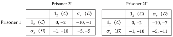
8.1.1. The Classical Version [30]

The classical Nash equilibrium is simple to find. Player type 2I has a dominant strategy of not confessing while type 2II has a dominant strategy to confess. Note also that in the game played between prisoner 1 and type 2II of prisoner 2, the strategy $\left(1_2,1_2\right)\to \left(C,C\right)$ is Pareto efficient. Assuming the two types of player 2 stick to their dominant strategies then if player 1 confesses he gets $-10\mu +0\left(1-\mu \right)$ while if he does not he gets $-5\mu -1\left(1-\mu \right)$ . Therefore, player 1 strategy is

$\begin{array}{l}\text{player}\text{1}\text{strategy}\\ =(\begin{array}{l}I\left(\text{confess}\right)\text{if}-10\mu +0\left(1-\mu \right)>-5\mu -1\left(1-\mu \right)\Rightarrow \mu <\frac{1}{6}\mathrm{,}\\ {\sigma }_x\left(\text{don}’\text{t}\text{confess}\right)\text{if}-10\mu +0\left(1-\mu \right)<-5\mu -1\left(1-\mu \right)\Rightarrow \mu >\frac{1}{6},\\ \text{indifferent}\text{if}\mu =\frac{1}{6}\mathrm{<mtext>\; \hspace{0.17em}\; </mtext>\; .}\end{array}\end{array}$ (71)

The Nash equilibrium and the corresponding “payoffs” are,

$\text{Nash}\text{equilibrium}=(\begin{array}{l}\left(I{\sigma }_{x}I\right)\to \left(CDC\right)\left(-10\mu \mathrm{,}-\mathrm{1,}-2\right)\mu <\frac{1}{6}\mathrm{,}\\ \left({\sigma }_x{\sigma }_{x}I\right)\to \left(DDC\right)\left(-1-4\mu \mathrm{,}-\mathrm{5,}-10\right)\mu >\frac{1}{6}\mathrm{.}\end{array}$ (72)

Henceforth, the game as defined above is referred to as the classical DA brother Bayesian game.

8.1.2. Definition of a Pure Strategy Quantum Bayesian Game

A formal definition of a quantum Bayesian game is now in order. Since we limit our formulation of classical games in terms of bits (and remembering that each bit can get two values 0 or 1), we will limit our discussion to quantum Bayesian games in which analogous classical games there are two possible decisions. Let

$G_{CB}=\langle N\mathrm{,}\left\{S_i\right\}\mathrm{,}\left\{u_i\left(\mathrm{.}\right)\right\}\mathrm{,}M\mathrm{,}F\left(\mathrm{.}\right)\mathrm{,}N=\left\{\mathrm{1,2,}\cdots ,n\right\}\mathrm{,}i=\mathrm{1,2,}\cdots \mathrm{,}n\mathrm{,}F\left(\mathrm{.}\right)\rangle \mathrm{<mtext>\; \hspace{0.17em}\; </mtext>\; ,}$ (73)

denote a classical Bayesian game. Here $S_i=\left(I_2\mathrm{,}{\sigma }_x\right)$ is the classical strategy set for player i, $u_i\left(s_i\mathrm{,}{s}_{-i}\mathrm{,}{\mu }_i\right)$ is a payoff function of player i where ${\mu }_i\in M_i$ is a random variable generated by nature that is observed only by player i. The joint probability distribution of ${\mu }_i$ , $F\left({\mu }_1\mathrm{,}{\mu }_2\mathrm{,}\cdots ,{\mu }_n\right)$ is a common knowledge and $M={\times }_{i=1}^n{M}_i$ . Then a pure strategy quantum Bayesian game is defined as,

$G_{QB}=\langle N\mathrm{,}\left\{{\gamma }_i\right\}\mathrm{,}\left\{u_i\left(\mathrm{.}\right)\right\}\mathrm{,}M\mathrm{,}F\left(\mathrm{.}\right)\mathrm{,}J\mathrm{,}{P}_i\mathrm{,}N=\left\{\mathrm{1,2,}\cdots ,n\right\}\mathrm{,}i=\mathrm{1,2,}\cdots \mathrm{,}n\mathrm{,}F\left(\mathrm{.}\right)\rangle \mathrm{<mtext>\; \hspace{0.17em}\; </mtext>\; ,}$ (74)

where the definitions to be modified compared with G_CB are as follows: 1) ${\gamma }_i=\left({\varphi }_i\mathrm{,}{\alpha }_i\mathrm{,}{\theta }_i\right)$ is the set of angles that determine the quantum strategy $U\left(\varphi ,{\alpha }_i\mathrm{,}{\theta }_i\right)$ according to Equation (18). 2) J is the entanglement operator fixed by the referee. 3) $P_i\left({\gamma }_i\mathrm{,}{\gamma }_{-i}\mathrm{,}{\mu }_i\right)$ are the payoff of player i determined by the quantum rules, see Equation (38) for $P_i$ defined for the full information game. A modification required for the Bayesian game is explicitly given below in Equation (77).

8.1.3. The DA brother Quantum Bayesian Game

Now let us concentrate on the quantum version of the DA brother Bayesian game. Our discussion here will focus on the general formulation and will not enter the discretization and numerical formalism. The strategies are determined by the three angles chosen by each player 1, 2I and 2II

${\gamma }_1=\left({\varphi }_1,{\alpha }_1,{\theta }_1\right),{\gamma }_{2I}=\left({\varphi }_{2I},{\alpha }_{2I},{\theta }_{2I}\right),{\gamma }_{2II}=\left({\varphi }_{2II},{\alpha }_{2II},{\theta }_{2II}\right).$ (75)

That leads according to Equation (18) to the three matrices $U\left({\gamma }_1\right)\mathrm{,}U\left({\gamma }_{2I}\right)\mathrm{,}$ $U\left({\gamma }_{2II}\right)$ . Each type of player 2, namely, 2I and 2II faces player 1 and the quantum game between them is conducted according to the rules specified in Section 3 especially Figure 3. Each game results in the corresponding final state (the subscripts should include also payer 1 but it is omitted for convenience)

$\begin{array}{l}|{\Psi }_{2I}\rangle =a_{2I}|00\rangle +b_{2I}|01\rangle +c_{2I}|10\rangle +d_{2I}|11\rangle ,\\ |{\Psi }_{2II}\rangle =a_{2II}|00\rangle +b_{2II}|01\rangle +c_{2II}|10\rangle +d_{2II}|11\rangle .\end{array}$ (76)

The coefficients in the expression for $|{\Psi }_{2I}\rangle$ depend on ${\gamma }_1\mathrm{,}{\gamma }_{2I}$ and the coefficients in the expression for $|{\Psi }_{2II}\rangle$ depend on ${\gamma }_1\mathrm{,}{\gamma }_{2II}$ . Explicit expressions for the coefficients depend on the entanglement operator J that is used by the referee. Below we will concentrate on the case of maximal entanglement matrix $J=J_1$ , with $J|00\rangle =|{\psi }^{+}\rangle$ as defined in Equations (31) and (47). The coefficients are given in Equation (50) wherein for player of type 2I the angles ${\varphi }_2\mathrm{,}{\alpha }_2\mathrm{,}{\theta }_2$ in Equation (50) are to be replaced by ${\varphi }_{2I}\mathrm{,}{\alpha }_{2I}\mathrm{,}{\theta }_{2I}$ and for player of type 2II the angles ${\varphi }_2\mathrm{,}{\alpha }_2\mathrm{,}{\theta }_2$ in Equation (50) are to be replaced by ${\varphi }_{2II}\mathrm{,}{\alpha }_{2II}\mathrm{,}{\theta }_{2II}$ . Following the expressions for the payoff function as in Equation (38) and the present game tables, the corresponding payoffs are,

$\begin{array}{l}{P}_{2I}\left({\gamma }_1;{\gamma }_{2I}\right)={\left|a_{2I}\right|}^2\times \left(-2\right)+{\left|b_{2I}\right|}^2\times \left(-1\right)+{\left|c_{2I}\right|}^2\times \left(-10\right)+{\left|d_{2I}\right|}^2\times \left(-5\right)\\ P_{2II}\left({\gamma }_1;{\gamma }_{2II}\right)={\left|a_{2II}\right|}^2\times \left(-2\right)+{\left|b_{2II}\right|}^2\times \left(-7\right)+{\left|c_{2II}\right|}^2\times \left(-10\right)+{\left|d_{2II}\right|}^2\times \left(-11\right)\\ P_1\left({\gamma }_1;{\gamma }_{2I},{\gamma }_{2II}\right)=\overline{{\left|a\right|}^2}\times 0+\overline{{\left|b\right|}^2}\times \left(-10\right)+\overline{{\left|c\right|}^2}\times \left(-1\right)+\overline{{\left|d\right|}^2}\times \left(-5\right)\\ \overline{{\left|a\right|}^2}=\mu {\left|a_{2I}\right|}^2+\left(1-\mu \right){\left|a_{2II}\right|}^2,\overline{{\left|b\right|}^2}=\mu {\left|b_{2I}\right|}^2+\left(1-\mu \right){\left|b_{2II}\right|}^2,\\ \overline{{\left|c\right|}^2}=\mu {\left|c_{2I}\right|}^2+\left(1-\mu \right){\left|c_{2II}\right|}^2,\overline{{\left|d\right|}^2}=\mu {\left|d_{2I}\right|}^2+\left(1-\mu \right){\left|d_{2II}\right|}^2.\end{array}$ (77)

8.1.4. Definition of a Pure Strategy Nash Equilibrium in Quantum Bayesian Game

We will define the pure strategy Nash equilibrium for the specific game under study, but a generalization to an arbitrary game as defined in Equation (74) is straightforward. A pure strategy Nash equilibrium for the quantum Bayesian game derived from the classical DA brother Bayesian game is the triple of strategies $\left({\gamma }_1^{\mathrm{<mo>\; *\; </mo>}}\mathrm{,}{\gamma }_{2I}^{\mathrm{<mo>\; *\; </mo>}}\mathrm{,}{\gamma }_{2II}^{\mathrm{<mo>\; *\; </mo>}}\right)$ (if it exists, recall that each $\gamma$ stands for three angles $\varphi \mathrm{,}\alpha \mathrm{,}\theta$ as in Equation (75)) that satisfies,

$\begin{array}{l}{P}_1\left({\gamma }_1,{\gamma }_{2I}^{*},{\gamma }_{2II}^{*}\right)\le P_1\left({\gamma }_1^{*},{\gamma }_{2I}^{*},{\gamma }_{2II}^{*}\right)\forall {\gamma }_1,\\ P_{2I}\left({\gamma }_1^{*},{\gamma }_{2I}\right)\le P_{2I}\left({\gamma }_1^{*},{\gamma }_{2I}^{*}\right)\forall {\gamma }_{2I},\\ P_{2II}\left({\gamma }_1^{*},{\gamma }_{2II}\right)\le P_{2I}\left({\gamma }_1^{*},{\gamma }_{2II}^{*}\right)\forall {\gamma }_{2II}.\end{array}$ (78)

8.1.5. Nash Equilibrium despite Maximal Entanglement

We have seen in subsection 4.4 that when J is leads to maximally entangled state $|{\psi }^{+}\rangle$ there is no pure strategy Nash equilibrium in the (full information) game played between player 1 and player 2I. One of the conditions for the proof of this negative result is that there is no Pareto efficient pure strategy Nash equilibrium in the classical game, which is indeed the case as far as the game between player 1 and player 2I is concerned. On the other hand, in the classical game played between players 1 and 2II the profile of strategies $1\otimes 1$ (both confess) is a Pareto efficient pure strategy Nash equilibrium. What can be said about the Quantum version? Intuitively, we expect that for small $\mu$ , player 2II will dominate and the game will have a pure strategy Nash equilibrium, but at some value of $\mu$ player 2I will dominate and there will be no equilibrium. We show below that this is indeed what happens, and that the critical value of $\mu$ is 1/6, that is exactly the value where, in the classical game, player 1 changes his strategy from $1$ (confess) to ${\sigma }_x$ (don’t confess).

From Equations (77) it is clear that for every strategy ${\gamma }_1$ player type 2I will seek his classical strategy and try to arrive at the situation where ${\left|b_{2I}\right|}^2=1$ , ${\left|a_{2I}\right|}^2={\left|c_{2I}\right|}^2={\left|d_{2I}\right|}^2=0$ , while player type 2II will seek his classical strategy and try to arrive at the situation where ${\left|a_{2II}\right|}^2=1$ , ${\left|b_{2I}\right|}^2={\left|c_{2I}\right|}^2={\left|d_{2I}\right|}^2=0$ . First let us check with the help of Equations (50) if they can indeed achieve it and then check the response of player 1.

Player 2I best response (he wants ${\left|b_{2I}\right|}^2=1$ ): According to Equation (50) we

have,

${\left|b_{2I}\right|}^2={\left[\cos \frac{1}{2}{\theta }_1\sin \frac{1}{2}{\theta }_{2I}\cos \left({\varphi }_1-{\alpha }_{2I}\right)+\sin \frac{1}{2}{\theta }_1\cos \frac{1}{2}{\theta }_{2I}\sin \left({\alpha }_1-{\varphi }_{2I}\right)\right]}^2$ .

Recall that for $\theta =0$ $\alpha$ is not defined and conventionally assumes the value 0. Similarly, for $\theta =\pi$ $\varphi$ is not defined and conventionally assumes the value 0. Therefore, by choosing

${\theta }_{2I}=\pi -{\theta }_1,{\alpha }_{2I}={\varphi }_1,{\varphi }_{2I}={\alpha }_1-\frac{\pi }{2}\text{modulo}2\pi$

player 2I gets, ${\left|b_{2I}\right|}^2={\left|\sin \frac{1}{2}\left({\theta }_1+{\theta }_{2I}\right)\right|}^2={\sin }^2\frac{\pi }{2}=1$ . The modulo 2π is optional in order to keep $0\le {\varphi }_{2I}<2\pi$ . Therefore the best response function of player 2I (that is a triple functions) is,

$q_{2I}\left({\gamma }_1\right)=q_{2I}\left({\varphi }_1,{\alpha }_1,{\theta }_1\right)=\left({\alpha }_1-\frac{\pi }{2},{\varphi }_1,\pi -{\theta }_1\right)\mathrm{<mtext>\; \hspace{0.17em}\; </mtext>\; .}$ (79)

Player 2II best response (he wants ${\left|a_{2II}\right|}^2=1$ ): According to Equation (50) we have,

${\left|a_{2II}\right|}^2={\left[\cos \frac{1}{2}{\theta }_1\cos \frac{1}{2}{\theta }_{2II}\cos \left({\varphi }_1+{\varphi }_{2II}\right)-\sin \frac{1}{2}{\theta }_1\sin \frac{1}{2}{\theta }_{2II}\sin \left({\alpha }_1+{\alpha }_{2II}\right)\right]}^2$ ,

Therefore, by choosing

${\theta }_{2II}={\theta }_1,{\varphi }_{2II}=-{\varphi }_1\text{modulo}2\pi ,{\alpha }_{2II}=-\left({\alpha }_1+\frac{\pi }{2}\right)\text{modulo}2\pi$

player 2II gets, ${\left|a_{2II}\right|}^2={\left|\cos \frac{1}{2}\left({\theta }_1-{\theta }_{2II}\right)\right|}^2=1$ . Therefore the best response function of player 2II (that is a triple functions) is,

$q_{2II}\left({\gamma }_1\right)=q_{2II}\left({\varphi }_1\mathrm{,}{\alpha }_1\mathrm{,}{\theta }_1\right)=\left(-{\varphi }_1\mathrm{,}-\left({\alpha }_1+\frac{\pi }{2}\right)\mathrm{,}{\theta }_1\right)\mathrm{<mtext>\; \hspace{0.17em}\; </mtext>\; .}$ (80)

Finding the best response function of player 1, $q_1\left({\gamma }_{2I}\mathrm{,}{\gamma }_{2II}\right)$ is virtually hopeless. However, guided by the classical game results, we are tempted to test whether, for small $\mu$ , the first player will choose his classical strategy ${\gamma }_1=\left(\mathrm{0,0,0}\right)$ which means that his 2 × 2 strategy matrix is $1$ . In that case, the best response functions of players 2I and 2II are $q_{2I}\left(\mathrm{0,0,0}\right)$ and $q_{2II}\left(\mathrm{0,0,0}\right)$ where the functions are defined in Equations (79) and (80). In other words, we have

Proposition: For $\mu \le 1/6$ , a pure strategy Nash equilibrium of the Bayesian quantum game is the “triple of triples”

$\left({\gamma }_1^{\mathrm{<mo>\; *\; </mo>}}\mathrm{,}{\gamma }_{2I}^{\mathrm{<mo>\; *\; </mo>}}\mathrm{,}{\gamma }_{2II}^{\mathrm{<mo>\; *\; </mo>}}\right)=\left[\left(\mathrm{0,0,0}\right)\mathrm{,}{q}_{2I}\left(\mathrm{0,0,0}\right)\mathrm{,}{q}_{2II}\left(\mathrm{0,0,0}\right)\right]\mathrm{<mtext>\; \hspace{0.17em}\; </mtext>\; .}$ (81)

Proof By construction, ${\gamma }_{2I}^{\mathrm{<mo>\; *\; </mo>}}$ and ${\gamma }_{2II}^{\mathrm{<mo>\; *\; </mo>}}$ are best responses to ${\gamma }_1^{\mathrm{<mo>\; *\; </mo>}}$ and therefore,

$P_{2I}\left({\gamma }_1^{\mathrm{<mo>\; *\; </mo>}}\mathrm{,}{\gamma }_{2I}\right)\le P_{2I}\left({\gamma }_1^{\mathrm{<mo>\; *\; </mo>}}\mathrm{,}{\gamma }_{2I}^{\mathrm{<mo>\; *\; </mo>}}\right)\forall {\gamma }_{2I}$ $P_{2II}\left({\gamma }_1^{\mathrm{<mo>\; *\; </mo>}}\mathrm{,}{\gamma }_{2II}\right)\le P_{2II}\left({\gamma }_1^{\mathrm{<mo>\; *\; </mo>}}\mathrm{,}{\gamma }_{2II}^{\mathrm{<mo>\; *\; </mo>}}\right)\forall {\gamma }_{2II}$

To check for $P_1$ we use Equation (77) and recall the expression for the coefficients from Equation (50). For any ${\gamma }_1=\left({\varphi }_1\mathrm{,}{\alpha }_1\mathrm{,}{\theta }_1\right)$ we find, after some calculations,

$\begin{array}{l}{P}_1\left({\varphi }_1\mathrm{,}{\alpha }_1\mathrm{,}{\theta }_1\mathrm{,}{\gamma }_{2I}^{\mathrm{<mo>\; *\; </mo>}}\mathrm{,}{\gamma }_{2II}^{\mathrm{<mo>\; *\; </mo>}}\right)\\ =-10\left[\mu {\left(\cos \frac{1}{2}{\theta }_1\cos {\varphi }_1\right)}^2+\left(1-\mu \right){\left(\sin \frac{1}{2}{\theta }_1\sin {\alpha }_1\right)}^2\right]\\ -\left[\mu {\left(\cos \frac{1}{2}{\theta }_1\sin {\varphi }_1\right)}^2+\left(1-\mu \right){\left(\sin \frac{1}{2}{\theta }_1\cos {\alpha }_1\right)}^2\right]\\ -5\left[\mu {\left(\sin \frac{1}{2}{\theta }_1\cos {\alpha }_1\right)}^2+\left(1-\mu \right){\left(\cos \frac{1}{2}{\theta }_1\sin {\varphi }_1\right)}^2\right]\mathrm{<mtext>\; \hspace{0.17em}\; </mtext>\; .}\end{array}$ (82)

Although finding a global maximum of a function of three continuous variables is not an easy task, all my numerical test indicates that for $\mu \le \frac{1}{6}$ , the payoff $P_1\left({\varphi }_1\mathrm{,}{\alpha }_1\mathrm{,}{\theta }_1\mathrm{,}{\gamma }_{2I}^{\mathrm{<mo>\; *\; </mo>}}\mathrm{,}{\gamma }_{2II}^{\mathrm{<mo>\; *\; </mo>}}\right)$ of player 1 has a global maximum at $\left({\varphi }_1\mathrm{,}{\alpha }_1\mathrm{,}{\theta }_1\right)=\left(\mathrm{0,0,0}\right)$ with payoff value $-10\mu$ . Thus, for $\mu \le 1/6$ the classical and quantum payoffs are identical, $\left(P_1\mathrm{,}{P}_2\mathrm{,}I\mathrm{,}{P}_{2II}\right)=\left(-10\mu \mathrm{,}-\mathrm{1,}-2\right)$ . On the other hand, for $\mu >1/6$ it is easy to show that $P_1$ as defined in Equation (82) does not have a global maximum at $\left(\mathrm{0,0,0}\right)$ and as my numerical algorithm indicates, the quantum version of the DA brother Bayesian game with maximal entanglement does not have a pure strategy Nash equilibrium.

9. Two-Players Three Strategies Games

Note: This section is based on the concepts reported in Ref. [34] wherein an entanglement operator is constructed for the system of two-players N strategies quantum game. The unavoidable overlap is included for the sake of self-consistence.

So far, all our analysis was constructed upon classical games with two strategies per each player. These two strategies are represented by 2 × 2 matrices $1=\left(\begin{array}{cc}1& 0\\ 0& 1\end{array}\right)$ and ${\sigma }_x=\left(\begin{array}{cc}0& 1\\ 1& 0\end{array}\right)$ that operate on the two bit states represented as vectors $|0\rangle =\left(\begin{array}{c}1\\ 0\end{array}\right)$ and $|1\rangle =\left(\begin{array}{c}0\\ 1\end{array}\right)$ . In this section, we will briefly touch upon the topic of quantum games based on 2-players 3-strategies classical game. The reason for carrying out this analysis is to check whether, in these structures there are special interesting features whose elucidation makes it worth to study despite the augmented complication. First, in subsection 9.1, we will describe how to cast the classical game in quantum information format, and define the notion of trits and classically non-commuting strategies. Then, in subsection 9.2, we will analyze the construction of the quantum game and define the notion of qutrits and quantum strategies as 3 × 3 matrices forming the group SU(3).

9.1. Two Players Three Strategies Classical Games: Trits

Now consider a two-players classical game with three strategies for each player. For example, prisoners may have three options: C, S and D for confess, Stay quiet or Don’t confess. In analogy with the bit notation 0, 1, these three options that are marked by 1, 2, 3 respectively, or in our ket notation $|1\rangle ,|2\rangle ,|3\rangle$ .

An object or a state that can assume three values is referred to as trit.

In analogy with the two-component vector notation for bits, we have,

$\text{trit}\text{state}1=\left(\begin{array}{c}1\\ 0\\ 0\end{array}\right)=|1\rangle ,\text{trit}\text{state}2=\left(\begin{array}{c}0\\ 1\\ 0\end{array}\right)=|2\rangle ,\text{trit}\text{state}3=\left(\begin{array}{c}0\\ 0\\ 1\end{array}\right)=|3\rangle .$ (83)

Similarly to Equations (3) and (4) we define two trit states as nine components vectors obtained by a Kronecker product of the two trits. Briefly, two-trit states are denoted as, $|ij\rangle =|i\rangle \otimes |j\rangle$ , $i,j=1,2,3$ . Note that for $i\ne j$ $|i\rangle \otimes |j\rangle \ne |j\rangle \otimes |i\rangle$ . The game table consists of two rows and three columns. The protocol of the classical game with 2-player and 3-strategies is similar (but not identical) to that of the 2-players 2-decision game. To underline the difference suppose that the judge calls the prisoners and tells them he assumes that they are in a two-trit state $|12\rangle$ meaning (C, S) namely, prisoner 1 confesses and prisoner 2 stays quiet. He then asks them to decide whether to leave their trit state as it is on $|1\rangle$ and $|2\rangle$ or to change it. These replacement operations are the players strategies. Since trits are represented by three component vectors, operation on trits (gates) is represented by 3 × 3 matrices. Unlike the case for two-players two strategies game where the states are bits, and the operations (strategies) are identical for both players, exhausted by $1_2$ (the unit 2 × 2 matrix) and ${\sigma }_x$ , the situation of the two players in the present game is different: For player 1, the strategies are $1_3$ (the 3 × 3 unit matrix leaving the trit as it is), S₁₂ (swapping of $|1\rangle$ and $|2\rangle$ namely, replacing C by S) and S₁₃ (swapping $|1\rangle$ and $|3\rangle$ namely replacing C by D). For player 2, the strategies are $1_3$ S₂₁ (swapping of $|2\rangle$ and $|1\rangle$ namely, replacing S by C) and S₂₃ (swapping $|2\rangle$ and $|3\rangle$ namely replacing S by D). In matrix notations the four operations are,

$1_3=\left(\begin{array}{ccc}1& 0& 0\\ 0& 1& 0\\ 0& 0& 1\end{array}\right),S_{12}=\left(\begin{array}{ccc}0& 1& 0\\ 1& 0& 0\\ 0& 0& 1\end{array}\right),S_{13}=\left(\begin{array}{ccc}0& 0& 1\\ 0& 1& 0\\ 1& 0& 0\end{array}\right),S_{23}=\left(\begin{array}{ccc}1& 0& 0\\ 0& 0& 1\\ 0& 1& 0\end{array}\right)$ (84)

These four matrices form a subset of $P_3$ , that is a representation of the permutations group on three objects that has six matrices. The other two matrices are such that all three elements change their place like $1\to 2\to 3\to 1$ (they do not have 1 on the diagonal) but they are not used in a simultaneous game with a single move. Thus, the four operations $1_3\mathrm{,}{S}_{12}\mathrm{,}{S}_{13}\mathrm{,}{S}_{23}$ do not form a group. Unlike the case of two-players two-strategies game where the two operations $1_2$ and ${\sigma }_x$ commute with each other, $\left[1_3\mathrm{,}{\sigma }_x\right]=0$ , here the strategies $S_{ij}$ do not commute with each other, for example,

$\left[S_{12}\mathrm{,}{S}_{13}\right]=S_{12}{S}_{13}-S_{13}{S}_{12}\ne \mathrm{0,}\text{etc}\mathrm{.}$ (85)

9.2. Qutrits

In this section we will briefly introduce the notion of quantum trits (qutrits) and quantum strategies in the quantum version of a two-players three-decisions game. This will mainly include a few definitions and some basic properties, since the analysis of such quantum game is too complicated and naturally falls beyond the scope of this research.

In order to define a qutrit we consider a three dimensional Bloch sphere S³ in which the three states of a trit, $|0\rangle ,|1\rangle$ and $|2\rangle$ are described by a point on its surface. This means that 1) Every element (vector, or ket) $|\psi \rangle \in S^3$ is expressible as a linear combination

$|\psi \rangle =v_1|1\rangle +v_2|2\rangle +v_3|3\rangle ,\text{where}{v}_1,v_2,v_3\in ℂ\mathrm{<mtext>\; \hspace{0.17em}\; </mtext>},{\left|v_1\right|}^2+{\left|v_2\right|}^2+{\left|v_3\right|}^2=1,$ (86)

recall that for qubit, $\left(\begin{array}{c}a\\ b\end{array}\right)$ we have ${\left|a\right|}^2+{\left|b\right|}^2=1$ . Thus,

Definition: A qutrit is a vector $|\psi \rangle =v_1|1\rangle +v_2|2\rangle +v_3|3\rangle \in S^3$ such that ${\left|v_1\right|}^2+{\left|v_2\right|}^2+{\left|v_3\right|}^2=1$ . In analogy with Equation (15), the representation of qutrits in terms of angular variables reads,

$|\psi \rangle ={\text{e}}^{i\alpha }\sin \theta \cos \varphi |1\rangle +{\text{e}}^{i\beta }\sin \theta \sin \varphi |2\rangle +\cos \theta |3\rangle \mathrm{<mtext>\; \hspace{0.17em}\; </mtext>\; .}$ (87)

9.2.1. Operations on Qutrits: Strategies

Instead of the 2 × 2 unitary matrix U defined in Equation (18) as a players strategy in the two players-two strategies game, a strategy of a player in a three strategies game is a unitary 3 × 3 complex matrix U with unit determinant det[U] = 1. The (infinite) set of all these matrices form a group, referred as the $SU\left(3\right)$ group. It plays a central role in physics especially in the classification of elementary particles. Unlike the two-strategies game where the 2 × 2 strategy matrices $U\left(\varphi \mathrm{,}\alpha \mathrm{,}\theta \right)\in SU\left(2\right)$ depend on three Euler angles, the quantum strategies $U\in SU\left(3\right)$ in the three strategies game depend on eight Euler angles, $U\left({\alpha }_1\mathrm{,}{\alpha }_2\mathrm{,}\cdots \mathrm{,}{\alpha }_8\right)\in SU\left(3\right)$ . That turns any attempt to use numerical approach virtually useless. Instead, we will list a few properties of the pertinent quantum game that indicates that it is principally different from the quantum game based on 2-players 2-strategies classical games.

9.2.2. Entanglment of Two Qutrit States

Like in the simpler quantum games based on 2-players 2-strategies, entanglement plays a crucial role also in 2-players 3-strategies games. First, let us define a two qutrit state and then define entanglement. A general two qutrit state (a point on S⁸) can be written as,

$|\Gamma \rangle ={\displaystyle \underset{i,j=1}{\overset{3}{\sum }}}{v}_{ij}|ij\rangle ,{\displaystyle \underset{i,j=1}{\overset{3}{\sum }}}{\left|v_{ij}\right|}^2=\mathrm{1\; <mtext>\; \hspace{0.17em}\; </mtext>\; .}$ (88)

Consider now two qutrits,

$|{\psi }_1\rangle ={\displaystyle \underset{i=1}{\overset{3}{\sum }}}{a}_i|i\rangle ,a_i\in ℂ,{\displaystyle \underset{i=1}{\overset{3}{\sum }}}{\left|a_i\right|}^2=1,|{\psi }_2\rangle ={\displaystyle \underset{j=1}{\overset{3}{\sum }}}{b}_j|j\rangle ,b_j\in ℂ,{\displaystyle \underset{j=1}{\overset{3}{\sum }}}{\left|b_j\right|}^2=\mathrm{1\; <mtext>\; \hspace{0.17em}\; </mtext>\; .}$ (89)

Their outer (or tensor) product is defined as,

$|{\psi }_1\rangle \otimes |{\psi }_2\rangle ={\displaystyle \underset{i,j=1}{\overset{3}{\sum }}}{a}_i{b}_j|ij\rangle \mathrm{<mtext>\; \hspace{0.17em}\; </mtext>\; .}$ (90)

Then we have:

Definition: A general 2 qutrits state $|\Gamma \rangle$ as defined in Equation (88) is said to be entangled if it cannot be written as an outer product of two qutrits as in Equation (90). We give (without proof) an example of maximally entangled two-qutrit states,

${|\Psi \rangle }_{\text{ME}}=\frac{1}{\sqrt{3}}\left(u_1|11\rangle +u_2|22\rangle +u_3|33\rangle \right)\mathrm{,}{u}_i\in ℂ\mathrm{,}\left|u_i\right|=\mathrm{1\; <mtext>\; \hspace{0.17em}\; </mtext>\; .}$ (91)

9.2.3. New Elements in Quantum Games Based on 2-Players 3-Strategies Classical Games

Suppose we try to organize the conduction of a quantum game based on a classical two-players three strategies game as a straightforward extension of the procedure used to quantize a two-players two strategies quantum game as displayed in Figure 3. The first move by the referee, that is, fixing an initial two-qutrit state (usually the classical two trit states $|11\rangle =\left(C\mathrm{,}C\right)$ ) is indeed identical. But the second operation, namely, operating by the entanglement operator is less straightforward because we first have to identify the maximally and partially entangled states in $S^3\otimes S^3$ and then to design the 9 × 9 matrix J that turns the non-entangled two qutrit initial state $|11\rangle$ into a maximally entangled state in analogy with Equation (31) or Equation (32). The maximally entangled state ${|\Psi \rangle }_{\text{ME}}$ has already been identified in Equation (91). In searching for an entanglement operator J such that $J|11\rangle ={|\Psi \rangle }_{\text{ME}}$ we recall an important and desirable property that we want to be satisfied by J, namely, classical commensurability. Mathematically it means that J should commute with all outer products of the classical strategies (see Equations (45) and (47) for the 2-players 2-strategies case). The reason for demanding classical commensurability is to assure that classical strategies are a special case of the quantum strategies as explained in connection with Equation (46).

Concentrating on the quantum game with initial state, $|11\rangle$ we then require

$J|11\rangle ={|\Psi \rangle }_{\text{ME}}\mathrm{,}\left[J\mathrm{,}{S}_{12}\otimes S_{13}\right]=\mathrm{0,}$ (92)

where the classical strategies are defined in Equation (84). A necessary and sufficient condition for satisfying Equation (92) will be composed of outer products of non-trivial 3 × 3 matrices that commute with both S₁₂ and S₁₃. But that is impossible as we now prove,

Theorem: In a quantum game based on 2-players 3-strategies classical game conducted as in Figure 3 with a non-trivial entanglement operator J (Namely, the state $J|11\rangle$ is entangled) there is no classical commensurability, namely, the classical strategies are not achieved as a special case of the quantum strategies.

Proof A necessary and sufficient condition for classical commensurability is a relaxed version of Equation 92, namely,

$J|11\rangle =|\text{Entangled}\text{State}\rangle \mathrm{,}\left[J\mathrm{,}{S}_{12}\otimes S_{13}\right]=0.$ (93)

The second equality is possible only if J is a function of $A\otimes A$ where A is a 3 × 3 matrix satisfying $\left[A,S_{12}\right]=\left[A,S_{13}\right]=0$ , and the first equality requires that A is not simply a multiple of the unit matrix $1_3$ . Therefore we need to prove the following.

lemma: If a 3 × 3 matrix A satisfies $\left[A,S_{12}\right]=\left[A,S_{13}\right]=0$ the $A=C{1}_3$ where $C\ne 0$ is a number.

Proof of the lemma: Although the lemma can be proved by brute force writing down the equation implied by the commutation relations, we choose a more elegant way mainly because it can be easily generalized to games with any finite number of strategies. The lemma will be proved in steps.

1. If $\left[A,S_{12}\right]=\left[A,S_{13}\right]=0$ then A commutes with any monomial of S₁₂ and S₁₃. For example, $\left[A,S_{12}^2\right]=A{S}_{12}^2-S_{12}A{S}_{12}=A{S}_{12}^2-A{S}_{12}^2=0$ and so on.

2. We have already stated that S₁₂ and S₁₃ are the matrices representing permutations on three elements, specifically,

$S_{12}\left(\begin{array}{c}1\\ 2\\ 3\end{array}\right)=\left(\begin{array}{ccc}0& 1& 0\\ 1& 0& 0\\ 0& 0& 1\end{array}\right)\left(\begin{array}{c}1\\ 2\\ 3\end{array}\right)=\left(\begin{array}{c}2\\ 1\\ 3\end{array}\right),S_{13}\left(\begin{array}{c}1\\ 2\\ 3\end{array}\right)=\left(\begin{array}{ccc}0& 0& 1\\ 0& 1& 0\\ 1& 0& 0\end{array}\right)\left(\begin{array}{c}1\\ 2\\ 3\end{array}\right)=\left(\begin{array}{c}3\\ 2\\ 1\end{array}\right).$ (94)

It is easily verified that simple monomials of S₁₂ and S₁₃ generate all the other permutations of three objects, altogether 6 elements (including the permutation $1_3\mathrm{<mo>\; :\; </mo>}\left(123\right)\to \left(123\right)$ ). Explicitly,

$S_{12}{S}_{13}=\left(\begin{array}{ccc}0& 1& 0\\ 0& 0& 1\\ 1& 0& 0\end{array}\right):\left(123\right)\to \left(231\right);S_{13}{S}_{12}=\left(\begin{array}{ccc}0& 0& 1\\ 1& 0& 0\\ 0& 1& 0\end{array}\right):\left(123\right)\to \left(312\right).$ (95)

$S_{12}{S}_{13}{S}_{12}=\left(\begin{array}{ccc}1& 0& 0\\ 0& 0& 1\\ 0& 1& 0\end{array}\right)=S_{23}:\left(123\right)\to \left(132\right).$ (96)

Therefore, according to 1), the matrix A commutes with all the six matrices representing the set S₃ of all permutations of three objects.

3. From group theory we know that S₃ is a (non-commutative) group containing 6 elements, and that the five matrices $S_{12}\mathrm{,}{S}_{13}\mathrm{,}{S}_{23}\mathrm{,}{S}_{12}{S}_{13}\mathrm{,}{S}_{13}{S}_{12}$ listed above together with the 3 × 3 unit matrix $1_3$ form an irreducible representation of S₃.

4. The Schure lemma in group theory states that if a matrix commutes with all the matrices that form an irreducible representation of a group, then this matrix is a multiple of the unit matrix. Hence $A=C{1}_3$ and the lemma is proved. □

9.2.4. Designing J₁

A natural question is whether we can find an entanglement operator J such that when it acts on the two qutrit state $|00\rangle$ it yields ${|\Psi \rangle }_{\text{ME}}$ of Equation (91) as specified in Equation (92). For two qubit states we defined the corresponding entanglement operator $J\left(\beta \right)$ in Equation (56). When it acts on two qubit state $|00\rangle$ it gives the state $|{\psi }_{+}\left(\beta \right)\rangle$ which, for $\beta =\pi /4$ gives the maximally entangled Bell state ${\psi }_{+}\left(\frac{\pi }{4}\right)$ of Equation (33). But with qutrits the design of J (a 9 × 9 matrix) is more complicated. To find it we note that in order to get the two qutrit state $|11\rangle$ from the qutrit state $|00\rangle$ we have to operate on $|00\rangle$ with $X\equiv \left[S_{12}{S}_{13}\right]\otimes \left[S_{13}{S}_{12}\right]$ , see definition in Equation (95), whereas in order to get the two qutrit state $|22\rangle$ from the qutrit state $|00\rangle$ we have to operate on $|00\rangle$ with $X^{\text{T}}\equiv \left[S_{13}{S}_{12}\right]\otimes \left[S_{12}{S}_{13}\right]$ , see definition in Equation (95). Consider the 9 × 9 matrix

$Z\equiv X+X^{\text{T}},\Rightarrow Z|00\rangle =|11\rangle +|22\rangle ,Z^2=Z+2\times 1_{9\times 9},$ (97)

where the last equality holds because $\left[X\mathrm{,}{X}^{\text{T}}\right]=0$ and $X{X}^{\text{T}}=1_{9\times 9}$ . Now let us define,

$J\left(\beta \right)={\text{e}}^{i\beta Z}=a\left(\beta \right)+b\left(\beta \right)Z,$ (98)

where the equality holds because $Z^2=Z+2\times 1_{9\times 9}$ and the expansion of the exponent yields only linear expression with Z. To get the coefficients $a\left(\beta \right)$ and $b\left(\beta \right)$ we perform derivative of both sides of Equation (98) and obtain,

$\begin{array}{c}{J}^{\prime }=a^{\prime }+b^{\prime }Z=iZ{\text{e}}^{i\beta Z}=iZ\left(a+bZ\right)=iaZ+ib{Z}^2\\ =iaZ+ib\left(Z+2\right)=i\left(a+b\right)Z+2ib.\end{array}$ (99)

Equating powers of Z we get a set of differential equations,

$a^{\prime }=2ib,b^{\prime }=i\left(a+b\right),a\left(0\right)=1,b\left(0\right)=0,\Rightarrow \left(\begin{array}{c}a\left(\beta \right)\\ b\left(\beta \right)\end{array}\right)={\text{e}}^{i\beta \left(\begin{array}{c}02\\ 11\end{array}\right)}\left(\begin{array}{c}1\\ 0\end{array}\right)\mathrm{<mtext>\; \hspace{0.17em}\; </mtext>\; .}$ (100)

The calculations of the exponent are easily done with the results

$a=\frac{1}{3}{\text{e}}^{-i\beta }\left({\text{e}}^{3i\beta }+2\right),b=\frac{1}{3}{\text{e}}^{-i\beta }\left({\text{e}}^{3i\beta }-1\right),$ (101)

Inserting these results in Equation (98) and using Equation (97) we get,

$J\left(\beta \right)|00\rangle =\frac{1}{3}{\text{e}}^{-i\beta }\left[\left({\text{e}}^{3i\beta }+2\right)|00\rangle +\left({\text{e}}^{3i\beta }-1\right)\left(|11\rangle +|22\rangle \right)\right]\mathrm{<mtext>\; \hspace{0.17em}\; </mtext>\; .}$ (102)

Maximal entanglements obtains when the absolute values of all three coefficients are equal, namely,

$\left|{\text{e}}^{3i\beta }+2\right|=\left|{\text{e}}^{3i\beta }-1\right|\Rightarrow \beta =\frac{2\pi }{9}=40˚\mathrm{.}$ (103)

Thus we have explicitly found the desired entanglement operator.

To summarize: Introducing the quantum game based on 2-player 3-classical strategies brings a few new elements,

1. Richer quantum information content through the interaction of qutrits.

2. Richer strategy content encoded by SU(3) matrices that depend on eight Euler angles.

3. Intricate entanglement pattern in 2-qutrit states.

4. Absence of classical commensurability. The classical strategies are not achieved as a special case of the quantum strategies because it is impossible to design an entanglement operator J that commutes with all the classical strategies.

5. A non-trivial entanglement operator $J\left(\beta \right)$ acting on two qutrits states such that for $\beta =\frac{2\pi }{9}$ the two qutrit state $J\left(2\pi /9\right)|00\rangle$ is maximally entangled.

Note added With the increasing development of Artificial Intelligence (AI) it is expected that it will soon play a role in quantum games [35] [36] [37] [38] .

Acknowledgements

This manuscript is based on the MA thesis of the author under the supervision of Professor Oscar Volij, as partial fulfillment of academic duties toward achieving second degree in Economics in the Department of Economics at Ben Gurion University [39] . I would like to thank Oscar for teaching me the (classical) theory of games, and for directing me during my studies. I would also like to thank the academic and administrative staff of the Department of Economics for their warm hospitality and high level teaching efforts during my studies. Thanks are due also to Professor Adam Brandenburger for occasional discussions during our overlap period in NYU-Shanghai University.

Notation List

· $\Gamma$ : Defining two players two strategies quantum game, with strategies C = Confess and D = Do not confess.

· $ℝ$ : The set of real numbers.

· $ℂ$ : The set of complex numbers.

· $1_2$ : The unit 2 × 2 matrix.

· ${\sigma }_x\mathrm{,}{\sigma }_y\mathrm{,}{\sigma }_z$ : The three Pauli matrices.

· $G_C$ : Formal definition of two players two strategies classical game.

· $u_{ij}$ : Elements of the payoff matrix.

· $S_1\mathrm{,}{S}_2$ : Strategies.

· $S_1^{\mathrm{<mo>\; *\; </mo>}}\mathrm{,}{S}_2^{\mathrm{<mo>\; *\; </mo>}}$ : Nash equilibrium strategies.

· $p\mathrm{,1}-p$ : Probabilities in mixed strategy game.

· $|\psi \rangle$ : A short notation for qubit or qutrit.

· $U\left(\varphi \mathrm{,}\alpha \mathrm{,}\theta \right)$ : An SU(2) matrix defined by three Euler angles.

· $S^n$ Bloch (unit sphere in $n+1$ space).

· $|T\rangle \mathrm{,}|S\rangle \mathrm{,}|{\psi }_{\pm }\rangle$ : Four Bell states with maximal entanglement.

· $\gamma$ : Degree of entanglement.

· $|\Psi \rangle$ Two qubit state.

· $\mathcal{U}$ : SU(4) matrix operating on two qubit states.

· $J\left(\beta \right)$ : Entanglement operator, where $0\le \beta \le \frac{\pi }{2}$ determines the degree of entanglement.

· $P_1\mathrm{,}{P}_2$ : Payoffs in a two-players two strategies quantum games.

· $G_Q$ : Formal definition of two players two strategies quantum game.

· ${\gamma }_1\mathrm{,}{\gamma }_2$ : Strategies in quantum game, depending on the choice of the three Euler angles.

· ${\gamma }_1^{\mathrm{<mo>\; *\; </mo>}}\mathrm{,}{\gamma }_2^{\mathrm{<mo>\; *\; </mo>}}$ : Nash equilibrium strategies in quantum game, depending on the choice of the three Euler angles.

· $q\left(\varphi \mathrm{,}\alpha \mathrm{,}\theta \right)$ : Best response function of a player in a quantum game.

· $I\left(k_{\varphi }\mathrm{,}{k}_{\alpha }\mathrm{,}{k}_{\theta }\right)$ : Lexicographic ordering of discrete strategies determined by the three Euler angles.

· $G_D$ : Formal definition of two players two strategies quantum game with discrete set of strategies.

· $G_{Q\mathrm{,}\text{mixed}}$ : Formal definition of two players two strategies quantum game with mixed strategies.

· $\rho \left(\varphi \mathrm{,}\alpha \mathrm{,}\theta \right)$ : Distribution of strategies in mixed strategy quantum games, depending on three Euler angle.

· $G_{CB}$ : Formal definition of a. classical Bayesian game.

· $G_{QB}$ : Formal definition of a quantum Bayesian game.

· $\mu \mathrm{,}\left(1-\mu \right)$ : Probabilities of a prisoner in a mixed Bayesian quantum game.

· $S_{ij}$ : Elements of the permutation group.

· $|\Gamma \rangle$ : Two qutrit states.

· $U\left({\alpha }_1\mathrm{,}{\alpha }_2\mathrm{,}\cdots \mathrm{,}{\alpha }_8\right)\in SU\left(3\right)$ : Strategies in two players three strategies quantum games, depending on 8 Euler angles.

Conflicts of Interest

The author declares no conflicts of interest regarding the publication of this paper.

References

[1]	Shannon, C.E. (1949) A Mathematical Theory of Communication. University of Illinois Press, Evanston.
[2]	Nash, J. (1950) The Bargaining Problem. Econometric, 18, 155-162. https://doi.org/10.2307/1907266
[3]	Nash, J.F. (1950) Equilibrium Points in N-Person Games. Proceedings of the National Academy of Sciences, 36, 48-49. https://doi.org/10.1073/pnas.36.1.48
[4]	Nash, J. (1950) Non-Cooperative Games. Ph.D. Thesis, Princeton University, Princeton.
[5]	Nash, J. (1951) Non-Cooperative Games. Annals of Mathematics, 54, 286-295. https://doi.org/10.2307/1969529
[6]	Nash, J. (1953) Two-Person Cooperative Games. Econometrica, 21, 128-140. https://doi.org/10.2307/1906951
[7]	von Neumann, J. and Morgenstern, O. (1953) Theory of Games and Economic Behavior. Princeton University Press, Princeton.
[8]	Shor, P.W. (1997) Polynomial Time Algorithms for Prime Factorization and Discrete Logarithms on a Quantum Computer. SIAM Journal on Computing, 26, Article 1484. https://doi.org/10.1137/S0097539795293172
[9]	Wiesner, S. (1983) Conjugate Coding. ACM SIGACT News, 15, 78-88. https://doi.org/10.1145/1008908.1008920
[10]	Ekert, A.K. (1991) Quantum Cryptography Based on Bell’s Theorem. Physical Review Letters, 67, 661-663. https://doi.org/10.1103/PhysRevLett.67.661
[11]	Goldenberg, L., Vaidman, L. and Wiesner, S. (1999) Quantum Gambling. Physical Review Letters, 82, 3356. https://doi.org/10.1103/PhysRevLett.82.3356
[12]	Vaidman, L. (1999) Variations on the Theme of the Greenberger-Horne-Zeilinger Proof. Foundations of Physics, 29, 615-630. https://doi.org/10.1023/A:1018868326838
[13]	Meyer, D. (1999) Quantum Strategies. Physical Review Letters, 82, 1052-1055. https://doi.org/10.1103/PhysRevLett.82.1052
[14]	Eisert, J., Wilkens, M. and Lewenstein, M. (1999) Quantum Games and Quantum Strategies. Physical Review Letters, 83, 3077-3080. https://doi.org/10.1103/PhysRevLett.83.3077
[15]	Eisert, J. and Wilkens, M. (2000) Quantum Games. Journal of Modern Optics, 47, 2543-2556. https://doi.org/10.1080/09500340008232180
[16]	Benjamin, S.C. and Hayden, P.M. (2001) Comment on “Quantum Games and Quantum Strategies”. Physical Review Letters, 87, Article ID: 069801. https://doi.org/10.1103/PhysRevLett.87.069801
[17]	Benjamin, S.C. and Hayden, P.M. (2001) Multi-Player Quantum Games. Physical Review A, 64, Article ID: 030301. https://doi.org/10.1103/PhysRevA.64.030301
[18]	Flitney, A.P. and Abbott, D. (2002) An Introduction to Quantum Game Theory. Fluctuation and Noise Letters, 2, R175-R18. https://doi.org/10.1142/S0219477502000981
[19]	Piotrowski, E.W. and Slaadkowski, J. (2003) An Invitation to Quantum Game Theory. International Journal of Theoretical Physics, 42, 1089-1099. https://doi.org/10.1023/A:1025443111388
[20]	Flitney, A.P. and Abbott, D. (2003) Advantage of a Quantum Player over a Classical One in 2 × 2 Quantum Games. Proceedings of the Royal Society of London. Series A: Mathematical, Physical and Engineering Sciences, A459, 2463-2474. https://doi.org/10.1098/rspa.2003.1136
[21]	Iqbal, A. (2005) Studies in the Theory of Quantum Games. arXiv: quant-ph/0503176.
[22]	Landsburg, S.E. (2004) Quantum Game Theory. Notices of the American Mathematical Society, 51, 394-399.
[23]	Piotrowski, E.W. and Sladkowski, J. (2002) Quantum Market Games. Physica A: Statistical Mechanics and Its Applications, 312, 208-216.
[24]	Piotrowski, E.W. (2004) Quantum Game Theory in Finance. arXiv: quant-phys/0406129.
[25]	Piotrowski, E.W. and Sladkowski, J. (2002) Quantum Bargaining Games. Physica A: Statistical Mechanics and Its Applications, 308, 391-401. https://doi.org/10.1016/S0378-4371(02)00592-7
[26]	Lambertini, L. (2000) Quantum Mechanics and Mathematical Economics Are Isomorphic. John von Neumann between Physics and Economics. http://www.dse.unibo.it/wp/370.pdf
[27]	von Neumann, J. and Morgenstern, O. (1953) Theory of Games and Economic Behavior. Princeton University Press, Princeton, NJ.
[28]	Landsburg, S.E. (2011) Nash Equilibria in Quantum Games. Proceedings of the American Mathematical Society, 139, 4423-4434. https://doi.org/10.1090/S0002-9939-2011-10838-4
[29]	Avishai, Y. (2012) Quantum Games: Numerical Approach. 2012 8th International Conference on Natural Computation, Chongqing, 29-31 May 2012, 898-903. https://doi.org/10.1109/ICNC.2012.6234560
[30]	Mas-Colell, A., Whinston, M.D. and Green, J.R. (1995) Microeconomic Theory. Oxford University Press, Oxford.
[31]	Chen, K.Y. and Hogg, T. (2006) How Well Do People Play a Quantum Prisoners Dilemma? Quantum Information Processing, 5, 43-67. https://doi.org/10.1007/s11128-006-0012-7
[32]	Cheon, T. and Iqbal, A. (2008) Bayesian Nash Equilibria and Bell Inequalities. Journal of the Physical Society of Japan, 77, Article ID: 024801. https://doi.org/10.1143/JPSJ.77.024801
[33]	Harsanyi, J.C. (1967) Games with Incomplete Information Played by “Bayesian” players, I-III Part I. The Basic Model. Management Science, 14, 159-182. https://doi.org/10.1287/mnsc.14.3.159
[34]	Avishai, Y. (2015) Constructing Entanglers in 2-Players—N-Strategies Quantum Game. Journal of Quantum Information Science, 5, 16-23. https://doi.org/10.4236/jqis.2015.51003
[35]	Miakisz, K., Piotrowski, E.W. and Sładkowski, J. (2006) Quantization of Games: Towards Quantum Artificial Intelligence. Theoretical Computer Science, 358, 15-22. https://doi.org/10.1016/j.tcs.2005.11.003
[36]	Zhang, W.R. (2013) Bipolar Quantum Logic Gates and Quantum Cellular Combinatorics-A Logical Extension to Quantum Entanglement. Journal of Quantum Information Science, 3, 93-105. https://doi.org/10.4236/jqis.2013.32014
[37]	Zhang, W.R. (2021) If AI Machine Cannot Think, Can QI Machine Think-from Negative Numbers to Quantum Intelligence for Mind-Light-Matter Unity. Quantum Machine Intelligence, 5, Article No. 14. https://doi.org/10.1109/JAS.2021.1003868
[38]	Zhang, W.R. (2021) Ground-0 Axioms vs. First Principles and Second Law: From the Geometry of Light and Logic of Photon to Mind-Light-Matter Unity-AI&QI. IEEE/CAA Journal of Automatica Sinica, 8, 534-553. https://doi.org/10.1109/JAS.2021.1003868
[39]	Avishai, Y. (2013) Some Topics in Quantum Games. arXiv: 1306.0284.