Loop Quantum Gravity Harmonic Oscillator

Edwin Eugene Klingman

Cybernetic Micro Systems, Inc., San Gregorio, CA, USA.

DOI: 10.4236/jmp.2023.149073                

Abstract

Attempts to unify Gravity Theory and Quantum Field Theory (QFT) under Loop Quantum Gravity Theory (LQG), are diverse; a dividing line between classical and quantum is sought with Schrödinger cat-state experiments. A Primordial Field Theory-based alternative is presented, and a gravity-based harmonic oscillator developed. With quantum theory applied at micro-scales and gravity theory at meso- and macro-scales, this scale-gap contributes to the conceptual problems associated with Loop Quantum Gravity. Primordial field theory, spanning all scales, is used to conceptually stretch key ideas across this gap. An LQG interpretation of the wave function associated with the oscillator is explained.

Keywords

Quantum Loop Gravity, Spacetime Ontology, Energy-Time Ontology, Harmonic Oscillator, Meso-Scale, Cat States, Gravitational Wave Function

1. Introduction

Two paramount contemporary issues in physics are: the search for a theory of quantum gravity in the absence of experimental results probing quantum gravitational effects [1] and determining the dividing line between classical and quantum physics in terms of the limits of validity of the quantum superposition principle [2] . In this paper we address first superposition concepts, then quantum gravity theories and finally we address the quantum harmonic oscillator formalism in the loop quantum gravity framework. All of the above are treated in the context of the incompatibility of general relativity theory and quantum theory. These topics are covered in the following order:

• Quantum issues: “Cat” states and wave function collapse.

• Gravity issues: intro to loop quantum gravity in primordial field theory.

• Gravitomagnetism: review of C-field analysis of kinetic energy.

• C-field analysis of the pendulum; wave aspects.

• Harmonic oscillator formalism in quantum theory.

• Formulation of the pendulum harmonic oscillator.

• Quantizing the pendulum.

• Summary and Discussion.

2. Quantum Issues Apart from Gravity

Loop Quantum Gravity (LQG) theory attempts to describe the quantum behavior of gravitational fields. Outside of LQG, attempts to find a dividing line between classical and quantum are known as “cat” states, after Schrödinger’s Cat. In 1957 Feynman presented a Gedanken experiment in which a coherent superposition of a massive particle in two different spatial locations, generated, e.g., by a particle in a coherent superposition of spin states entering a Stern-Gerlach apparatus, acts gravitationally with another mass. This has later been extended to discussing the possibility of finding macroscopic objects in two places at the same time. Actual experiments are more mundane. Hauer, et al., [3] note that the experimental generation of macroscopic superposition states has yet to be demonstrated. They non-linearly couple a tuned microwave cavity to a mechanical resonator, however, “to generate significant Wigner negativity is unattainable in current experiments.” Cat states reported by Bild, et al., [4] focus on transient motions in a quantum system consisting of a qubit coupled to a piezo-electric lattice, whose vibrations induce phonon modes whose interactions may vanish or decouple as the different decay modes evolve at different rates until mutually coupled oscillation is revived.

If the phonon mode and qubit are sufficiently prepared, their coherent interaction rapidly dephases. Hence the oscillations of the qubit population “collapse”. Between collapse and revival, the qubit and phonon mode disentangle from each other. The experiment observes coupled oscillations of qubit and phonon mode, with coherent exchange of energy quanta between the qubit and photon mode during the resonant interaction. Oscillation energy transferred from phonon to qubit exists in high $E$ field of the piezoelectric lattice.

Consider a coherent array of pendula, of varying lengths, whose time-lapse observations show what visually appears to come in and out of phase. Translated to the meso-scale, a cat state might imply that a pendulum oscillator exists at both extremes as a superposition of states. Rather than such “cat”-states of motion, in which macroscopic systems are in spatially separate locations at the same time, and are described by the superposition of wave functions, we focus on the superposition of the loop quantum gravity states described by

$\Psi \left(x,t\right)={\displaystyle {\sum }_{i=1}^n{\psi }_i\left(x_i,t\right)}$ (1)

where $x$ is the center-of-mass of the n-particles, $\Psi \left(x,t\right)$ = meso-scale, ${\psi }_i\left(x_i,t\right)$ = micro-scale. This paper examines a meso-scale model of fundamental physics, the harmonic oscillator, after first treating various relevant issues.

In 2017 Berenstein & Miller asked if topology and geometry can be measured by an operator measurement in quantum gravity [5] ; they claim that topology cannot be measured by operator. They enquire about the nature of observables in a quantum theory of gravity, where, by observables, they mean a Hermitian (linear) operator in the Hilbert space of states as is usual in quantum mechanics. In view of the many approaches to quantum gravity, many based on AdS/CFT Holographic theory variants, they ask if spacetimes in a corresponding set of geometries correspond to different space-time topologies. Furthermore,

“The set of states we are interested in forms a Hilbert space in its own right. Quantum mechanics is therefore valid and quantum questions can be answered unambiguously.”

A key assumption is that the set of these coherent states is over-complete, so every other state in the Hilbert space can be obtained by superposition of the family of states and point out that is a well-known fact for studying states of a finite number of harmonic oscillators.

Donadi, Ferialdi, and Bassi focus on collapse of the wave function, assuming that physical systems are associated with a wave function, ψ, and that collapse of this wave function is triggered by noise. In this paper we show that the collapse of our wave function is generated by interaction with gravity, in a manner compatible with their conclusion that collapsing the wave function in space must change the average momentum of the system (typically associated with the center of mass of the system.)

3. Introduction to Loop Quantum Gravity in Energy-Time Theory

Loop Quantum Gravity points in many directions, see Armas’ Conversations on Quantum Gravity [6] , but none are subject to unanimous agreement. At one extreme are atoms of geometry, with string theory, AdS/CFT and CDT (Causal Dynamical Triangulation) representing alternate approaches. This situation is due to gravity being based on Einstein’s “space-time” theory for a century, with gravity viewed as the metric which describes the curvature of space. An alternative, paradox-free theory of gravity in an “energy-time” framework supports the derivation of gravity from the primordial field. A century ago, deBroglie postulated the key physics underlying quantum theory, $p=h/\lambda$ , and Schrodinger postulated the operator equivalent, $p=-i\hslash \nabla$ which, of course has the same dimensions as $h/\lambda$ . Energy-time theory accepts deBroglie but, with Richard Feynman, Steven Weinberg and others, views geometry unnecessary as a means of understanding gravity. Much of LQG, as expounded by Rovelli [7] , is focused on applying quantum formalism to gravity as geometry, leading to, for example:

“… a tetrahedron can have a geometry that turns out to be a linear combination … of different volume eigenvalues. … (it is) intuitive to think about nodes not as sharp geometrical points, but as minimum ‘quantum blobs’ of space-time, which are all spatially connected.”

Quantum theory is a probabilistic formulation that predicts nothing physical, describing, at best, the distribution of probabilities over physical events; so we expect it to apply to energy-time theory of gravity. However, quantum field theory postulates a “field-per-particle” in a mattress/lattice context wherein creation operators stimulate an excitation in a field that represents the field-specific particle, which is terminated or absorbed by an annihilation operator, whereas in primordial field theory there is only one primordial field, from which all particles must evolve. Primordial field ontology [8] [9] [10] focuses on materiality of the gravitational field and density dependence of energy/momentum. This loop quantum gravity theory is based on Heaviside’s equations derived from the self-interaction of the primordial field:

$\nabla \psi =\psi \psi$ (2)

The primordial field equation operating on a parameterized field $\psi =\psi \left(\xi \right)$ has two immediate solutions: scalar: ${\nabla }_{\xi }={\partial }_{\xi }\Rightarrow {\partial }_{\xi }\psi \left(\xi \right)=-{\xi }^{-1}$ and vector: ${\nabla }_{\xi }={\partial }_{\xi }\Rightarrow {\nabla }_{\xi }\psi \left(\xi \right)={\xi }^{-1}$ . If we let ${\psi }_{\xi }=G\left(\xi \right)$ and ${\psi }_{\xi }=C\left(\xi \right)$ and (2) becomes:

$\left(\nabla +{\partial }_t\right)\left(G\left(r\right)+iC\left(t\right)\right)=\left(G\left(r\right)+iC\left(t\right)\right)\left(G\left(r\right)+iC\left(t\right)\right)$ (3)

which leads to Heaviside’s equations when energy terms $G^2+C^2\Rightarrow \rho$ and $C\times G\Rightarrow \rho v$ are substituted appropriately. Heaviside’s equations can be derived from Einstein’s field equations, but this is usually falsely interpreted as the “weak field approximation”. Derivation from the physics of the primordial field includes no mention of field strength; the equations are applicable at all field strengths, including the ultra-strong fields present at the big bang, which gave birth to the primordial field.

The energies involved in relativistic mass are rest mass, $m{c}^2$ and momentum $p$ . Circa 1893, Heaviside extended Newtonian gravity, based on analogy with Maxwell’s equations, with a key equation describing the circulation of the gravitomagnetic field, which we call the C-field:

$\nabla \times C=-p+\frac{\partial G}{\partial t}$ (4)

in natural units $c=g=\hslash =1$ (c is the speed of light, g is Newton’s gravitational constant, with $G$ being the gravitational field). Instead of momentum, here $p$ symbolizes momentum density:

$p=\frac{P}{{\displaystyle \int {\text{d}}^{3}x}}$ . (5)

Momentum used in the Hamiltonian is $P=m_{0}v={\displaystyle \int {\text{d}}^{3}x}\nabla \times C$ . That is, momentum equals the volume integral of the C-field circulation induced by the momentum density $p$ . We temporarily ignore change in gravitational field, $\frac{\partial G}{\partial t}$ , and consider only $\nabla \times C=-p$ . The force $F$ accelerating a rest mass will give rise to a change in circulation of the C-field:

$F~\text{d}p/\text{d}t=\frac{\text{d}}{\text{d}t}\left(\nabla \times C\right)$ ~ change in circulation (6)

The negative sign in Equation (4) is associated with the direction of circulation, that is, momentum density $p$ induces a left-handed circulation about the momentum. But when we apply the force formula, any negative sign associated with change in momentum density $\text{d}p/\text{d}t$ will have the same meaning as the Lenz’s Law of electromagnetic theory. Feynman remarked about the mystery of why things continue at the same velocity—acceleration increases the C-field circulation, while deceleration is opposed by existing circulation. The same applies to a particle “tunneling” through a finite potential barrier. The change in momentum as the particle begins to penetrate the barrier is opposed by the corresponding force associated with the change in circulation. The particle is effectively accelerated by the collapsing C-field circulation until the circulation disappears.

4. Review of C-Field Analysis of Kinetic Energy

Energy density of the electromagnetic field is $~\left(E^2+B^2\right)$ . If, in fact, the energy density of any physical field is assumed proportional to the square of the field strength, then the formula for C-field energy density is:

$\left(\frac{c^2}{g}\right)\left(C\cdot C\right)$ = C-field energy density (7)

Multiplying energy density by local volume we obtain the dimensional relation:

${\displaystyle \int {\text{d}}^{3}x}\left(\frac{c^2}{g}\right)\left(C\cdot C\right)\Rightarrow \left(l^3\right)\cdot \left(\frac{m}{l}\right)\left(\frac{1}{t^2}\right)=\frac{m{l}^2}{t^2}\approx m{v}^2$ . (8)

The C-field has been shown to be real, [11] and thus to have finite energy density, however this local energy density is not considered in any standard treatment of kinetic energy (of motion). If C-field energy is not kinetic energy, it must be added to kinetic energy in any real physical situation. If C-field circulation energy is kinetic energy; no new energy accounting is required.

We adopt a gravitomagnetic approach dual to geometric algebra treatments of Maxwell’s equations modeled on Arthur [12] , who develops D³⁺¹ and 4D models in detail. For D³⁺¹-Maxwell equation $\left(\nabla +{\partial }_t\right)F=J$ with F the field tensor and J the source, $J=\rho \left(1+v\right)$ ; then multiplying both sides by $\left(\nabla -{\partial }_t\right)$ we obtain:

$\left({\nabla }^2-{\partial }_t^2\right)F=\left(\nabla -{\partial }_t\right)J$ . (9)

In source-free space $J=0$ and Equation (9) becomes the wave equation, which, in terms of a plane wave, reduces to $\left(-k^2+{\omega }^2\right)F=0$ . Making use of natural units $g=c=\hslash =1$ and the quantum equivalents: momentum $p=\hslash k$ and $E=\hslash \omega =\hslash C$ , we obtain:

$\left(-k^2+{\omega }^2\right)\Rightarrow -p^2+C^2=0$ (10)

For unit mass this implies an equivalence between energy densities:

$\begin{array}{l}{p}^2=C^2\\ /\backslash \\ \text{kinetic}\text{C-field}\end{array}$ (11)

Kinetic energy is thus physically represented by energy of gravitomagnetic circulation induced by momentum $p$ . While almost every energy in physics is associated with a potential or energy field, kinetic energy may be unique in having no field correlate. Heaviside’s theory of gravitomagnetism implies that the essentially undefined mechanism of storage of energy of motion is actually C-field circulation energy, bringing our most basic energy into agreement with all other field energies. In addition, we assume that ether-as-local-gravity corresponds to the reality of a local absolute. So, velocities are referenced to the local gravity system; typically, the center of the Earth.

Heaviside Equation (4) relates gravitomagnetic field circulation to momentum density, defined in Equation (5), with linear momentum $P=mv$ . We assume $\text{d}G/\text{d}t=0$ and multiply Equation (6) by local volume ${\displaystyle \int {\text{d}}^{3}x}$ to obtain

${\displaystyle \int {\text{d}}^{3}x}\frac{\text{d}}{\text{d}t}\left(\nabla \times C\right)=-\frac{\text{d}P}{\text{d}t}$ , (12)

and since the order of integration is immaterial, then

$\frac{\text{d}}{\text{d}t}\left({\displaystyle \int {\text{d}}^{3}x}\nabla \times C\right)=-\frac{\text{d}P}{\text{d}t}$ . (13)

An integral on D³⁺¹ is potentially complex in nature, but Arfken [13] shows that sometimes the local integral of an infinitesimal volume is equal to

${\displaystyle \int {\text{d}}^{3}x}=\Delta x\Delta y\Delta z=\text{trivector}$ (14)

Thus, integration over a volume is sometimes equivalent to multiplying by the scaled volume. Next, we consider the mass flowing through an infinitesimal volume.

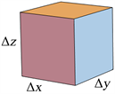
Sulejmanpasic [14] notes that the question of how a short-distance formulation of a given quantum theory is related to its long-distance physics is, in the most interesting cases, an extremely difficult one to understand. Ontologically, a cube of mass is not solid mass, but consists of atoms with electrons and nuclei. Clouds of electrons tend to keep the nuclei distributed evenly over local space but contribute very little to momentum density $\rho v$ where $\rho =\frac{m}{{\displaystyle \int {\text{d}}^{3}x}}$ and $m={\displaystyle \sum m_{nucleus}}$ . Figure 1(a) depicts a random distribution of nuclei moving in the same direction. C-field energy surrounding mass in motion, is shown around the individual nuclei; local field energy is largely contained inside the cube. Figure 1(b) shows two parallel momenta perpendicular to the plane of the page. Each momentum induces a left-handed C-field circulation, such that the fields cancel exactly half-way between the particles, while above and below the particles the field circulates more or less in the same direction, indicated by the arrows on the contour lines. If we place another momentum in the group, the appropriate circulation encloses all three particles. In fact, if we consider all of the momenta shown in Figure 1 in this way, we can envision the moving mass as surrounded by a circulating C-field.

While the C-field’s existence was proved in 2011 by Stanford’s Gravity Probe B experiment with results in good agreement with general relativity, the field in space is relatively weak, due to the low density of the Earth as seen from orbit. This result may seem to bring into question our analysis of the C-field-circulation-based kinetic energy of a pendulum. If one attempts to measure the C-field circulation outside of the pendulum bob or mass, one expects to find extremely weak C-field. But the kinetic energy of the mass is not found “outside” of the macro mass, which is physically constructed of electrons and nuclei. Electrons effectively flow in all directions and are negligible from our perspective. On the other hand, the nuclei, on average, are accelerated in the same direction and each extremely small nucleus contains most of the mass in the local neighborhood, resulting in very high mass density. C-field circulation is maximum surrounding the nuclear mass density, where it has the greatest Lenz Law-type effect on the mass. The energy of circulation of all the nuclei is additive.

That is, the C-field circulation that constitutes the kinetic energy of the pendulum is not found in the volume surrounding the bob, but is that surrounding every nucleus of which the mass consists. The Lenz-Law-like behavior relating the mass to acceleration and deceleration acts individually on every nucleus, not on the bob, per se; the sum of all nuclear C-field circulations constitutes the relevant kinetic energy of the bob, confirming that “relativistic mass” is the sum of rest mass, $m_0{c}^2$ , and kinetic energy, $\frac{1}{2}{m}_0{v}^2$ . The “storage mechanism” for kinetic energy of motion is seen to be gravitomagnetic circulation induced by the mass density in motion, i.e., momentum density.

(a) (b)

Figure 1. (a) Random atomic nuclei with common momentum density vectors distributed in local cube. (b) The C-field is summed around two nuclei with parallel momentum, perpendicular to the page. C-field cancellation occurs at the midpoint, but circulation around both particles form left-handed loops. The asymmetry is an artifact of the sampling instruction used to create the plot.

5. C-Field Analysis of the Pendulum—Wave Aspects

Apply the C-field circulation Equation (4) to the simple mechanical pendulum. Here, key to showing that the C-field energy is identically equal to kinetic energy is through use of $r\times p$ . The pendulum string is inelastic, so mass (m) cannot move in the $r$ direction, that is, $\text{d}r=0$ , but moves in the θ direction; $\left|v\right|~r\text{d}\theta /\text{d}t$ . From Heaviside’s equation,

$\nabla \times C=-\left(\frac{g}{c^2}\right)\rho v\left(t\right)$ (15)

As pendulum velocity varies, so does C-field circulation; based on the inverse curl operation [15] we obtain

${\left(\nabla \times \right)}^{-1}\left(\nabla \times \right)C=-\left(\frac{g\rho }{c^2}\right){\left(\nabla \times \right)}^{-1}v\Rightarrow C=\left(\frac{g\rho }{c^2}\right)r\times v$ (16)

which is geometrically correct at every step of motion. Next, square both sides:

$C\cdot C={\left(\frac{g\rho }{c^2}\right)}^2\left(r\times v\right)\cdot \left(r\times v\right)$ (17)

Since ${\left|r\times v\right|}^2+{\left|r\cdot v\right|}^2={\left|r\right|}^2{\left|v\right|}^2$ we have:

$\left(\frac{c^2}{g}\right)C\cdot C=\left(\frac{g}{c^2}\right){\rho }^2{r}^2{v}^2$ (18)

The left-hand-side of (18) is C-field energy density, and a dimensional analysis of the right-hand-side yields $\frac{m{v}^2}{l^3}$ , which has dimensions of kinetic energy over volume, i.e., energy density:

$\left\{\begin{array}{c}\text{Cfield}\\ \text{energy}\\ \text{density}\end{array}\right\}\iff \left\{\begin{array}{c}\text{kinetic}\\ \text{energy}\\ \text{density}\end{array}\right\}$

A note on notation: Most university physics ignores the gravitomagnetic field and labels the local gravitational field $g$ and Newton’s gravitational constant G. In our equations the gravitational field is $G$ and Newton’s constant is g. The pendulum is typically not analyzed in terms of the C-field, but in terms of the local $G$ field. An object falling from height $h=\Delta z$ will acquire kinetic energy ( $\Delta K=\frac{1}{2}m{v}^2$ ) that is equal to gravitational potential energy ( $\Delta U=mGh$ ) lost in the fall. The string from which the mass is suspended will not stretch, so the fall is not vertical. Nevertheless, the gravitational potential energy is converted to kinetic energy of motion along the arc $s=r\text{d}\theta$ . Since $\frac{1}{2}m{v}^2=mGh$ we have velocity $v=\sqrt{2Gh}$ . The velocity along the arc $\frac{\text{d}s}{\text{d}t}=\frac{\text{d}}{\text{d}t}\left(r\text{d}\theta \right)$ and the pendulum length does not change ( $\text{d}r=0$ ), so

$\frac{\text{d}s}{\text{d}t}=r\frac{\text{d}\theta }{\text{d}t}\Rightarrow \frac{\text{d}\theta }{\text{d}t}=\frac{\sqrt{2Gh}}{r}$ (19)

Use these relations for C-field circulation:

$\nabla \times C=-\left(\frac{g}{c^2}\right)\rho v+\frac{1}{c^2}\frac{\text{d}G}{\text{d}t}$ . (20)

The gravitational field $G~9.8\text{m}/{\text{sec}}^{\text{2}}$ is effectively constant at the surface of the Earth, hence $\text{d}G/\text{d}t=0$ . Since rest mass m does not change, instantaneous momentum $P=mv=m\sqrt{2G\Delta z}$ , where ∆z ranges from 0 to h. We are interested in momentum density $p=\frac{P}{{\displaystyle \int {\text{d}}^{3}x}}$ thus the integrated induced circulation equation becomes:

${\displaystyle \int {\text{d}}^{3}x}\left(\nabla \times C\right)=-\left(\frac{g}{c^2}\right)m\sqrt{2G\Delta z}$ . (21)

Our goal is to show that the kinetic energy $\frac{1}{2}m{v}^2=mGh$ is exactly equal to the C-field circulation, since we claim that the instantiation of the C-field is the kinetic energy. For the displaced pendulum $\theta ~{15}^{\circ }~\frac{\pi }{12}$ , the kinetic energy is initially zero, hence $\nabla \times C=0$ . For maximum velocity (at $\theta =0$ ) we have $v=\sqrt{2Gh}$ so that the induced circulation is

$\nabla \times C=-\left(\frac{g}{c^2}\right)\frac{m}{{\displaystyle \int {\text{d}}^{3}x}}\sqrt{2Gh}\equiv -\left(\frac{g}{c^2}\right)\rho v$ (22)

which leads to Equation (15), while identically equal to Heaviside’s C-field circulation equation.

Not obvious from the equations is that the period of the pendulum is independent of the initial displacement. A greater displacement yields a larger restoring force and hence a proportional increase in the acceleration (of falling), with greater velocity at zero displacement. The mass cancels out of the period, i.e., heavier masses do not change the period: $T=2\pi \sqrt{L/G}$ . The initial fall accelerates the mass with consequent change of momentum with time; $\text{d}p/\text{d}t$ increases. But since C-field circulation is proportional to momentum (density), change in momentum yields change in circulation, given by Equation (6). Once passed through $\theta =0$ , the mass is climbing against gravity, converting kinetic energy stored as C-field circulation into gravitational potential energy as it rises. The change of sign decreases the C-field circulation and hence the inertia, which is the key property of the field, see Figure 2. At maximum displacement the gravitational field essentially “collapses” the C-field wave function.

6. Harmonic Oscillator Formalism in Quantum Theory

The harmonic oscillator is one of the most basic and useful soluble examples in non-relativistic quantum mechanics [16] . The oscillator has an infinite number of bound states whose energies are equally spaced. Perhaps most significantly, the coherent wave packet oscillates exactly like its classical counterpart. Although relativistic harmonic oscillators are addressed, the behavior of the Dirac-based [ $H=\alpha p+\beta \left(m+S\left(x\right)\right)$ ] treatment, in most cases, is very similar to

(a) (b) (c)

Figure 2. (a) Start of swing. (b) Mid-swing. (c) Ending swing. The circulation is shown schematically in red over the entire path of the pendulum swings to represent the envelope of the field over the path. For more instantaneous values of the field, compare to Figure 3 and Figure 4.

the Schrödinger coherent wave packet of the non-relativistic harmonic oscillator, both governed by

$H{\psi }_i=E{\psi }_i$ (23)

Of course, rest mass counts as a key part of the relativistic energy for most mechanical oscillations [ $m\ddot{x}+kx=0$ ] yet the gravity-based restoring force is mass-independent [ $m\ddot{x}+mG\left(\theta \right)=0$ ], where the force is a function of angle θ. The Dirac solution, normally interpreted as representing both positive and negative energies, in most cases reduces to two Schrödinger equations:

$H_i{\psi }_i=\left[\frac{{\left(-i\hslash \nabla \right)}^2}{2m}+U_i\right]{\psi }_i=E_i{\psi }_i$ , (24)

only one of which is of interest to us.

In quantum field theory, Zee observes [17] that in non-relativistic QM the interaction between radiation and atoms is treated in terms of the electromagnetic field and its Fourier components are quantized as a collection of harmonic oscillators, leading to creation and annihilation operators for photons, but not electrons. Relativistic QM treats electrons and photons as elementary particles on the same footing. To demonstrate this we follow Griffiths, [18] for whom the paradigm for the classical harmonic oscillator is a mass m attached to a spring of force constant k, with motion governed by Hooke’s law, $F=-kx=m\ddot{x}$ with solutions $x\left(t\right)=A\sin \left(\omega t\right)+B\cos \left(\omega t\right)$ . Here frequency of oscillation, $\omega =\sqrt{k/m}$ and potential energy $\frac{1}{2}k{x}^2$ . The quantum problem is to solve the Schrödinger equation for the potential $V\left(x\right)=\frac{1}{2}m{\omega }^2{x}^2$ :

$\frac{-{\hslash }^2}{2m}\frac{{\text{d}}^2\psi }{\text{d}{x}^2}+\frac{1}{2}m{\omega }^2{x}^2\psi =E\psi$ (25)

Two approaches exist in the literature, but Griffiths finds the algebraic method of interest since it produces “ladder” operators. Based on $p=-i\hslash \nabla$ he rewrites Equation (25) to derive

$H=\frac{1}{2m}\left[p^2+\left(m^2{\omega }^2{x}^2\right)\right]$ (26)

Expanding (27) as $p^2+\left(m^2{\omega }^2{x}^2\right)=\left(ip+m\omega x\right)\left(-ip+m\omega x\right)$ and then defines the operator:

$a_{\pm }\equiv \frac{1}{\sqrt{2\hslash m\omega }}\left(\mp ip+m\omega x\right)$ (27)

with product

$a_{-}{a}_{+}=\frac{1}{2\hslash m\omega }\left[p^2+{\left(m\omega x\right)}^2-im\omega \left(xp-px\right)\right]$ . (28)

Defining the commutator operation $\left[x,p\right]=i\hslash$ he derives

$a_{-}{a}_{+}=\frac{1}{\hslash \omega }H-\frac{1}{2}$ (29)

and with $\left[a_{-},a_{+}\right]=1$

$H=\hslash \omega \left(a_{-}{a}_{+}-\frac{1}{2}\right)$ or $H=\hslash \omega \left(a_{+}{a}_{-}+\frac{1}{2}\right)$ (30)

which leads to

$\hslash \omega \left(a_{-}{a}_{+}-\frac{1}{2}\right)\Psi =E\Psi$ (31)

If $\Psi$ satisfies the Schrödinger equation with energy E, ( $H\Psi =E\Psi$ ), then $a_{+}\Psi$ satisfies the Schrödinger equation with $E+\hslash \omega$ , i.e.,

$H\left(a_{+}\Psi \right)=\left(E+\hslash \omega \right)\left(a_{+}\Psi \right)$ (32)

and by the same token

$H\left(a_{-}\Psi \right)=\left(E-\hslash \omega \right)\left(a_{-}\Psi \right)$ (33)

These raising and lowering operators (or ladder operators) provided that, if we can find one solution $\Psi$ , we can generate other solutions through application of these operators. In practice, there is a “lowest rung” on the ladder such that $a_{-}\Psi =0$ . This allows us to solve for

${\psi }_i\left(x\right):\frac{1}{\sqrt{2\hslash m\omega }}\left(\hslash \frac{\text{d}}{\text{d}x}+m\omega x\right){\psi }_0=0$ (34)

which leads to

${\psi }_0\left(x\right)=A{\text{e}}^{\frac{-m\omega }{2\hslash }{x}^2}$

by repeatedly applying the raising operator to generate excited states, the energy increases by $\hslash \omega$ with each step.

${\psi }_n\left(x\right)=A_n{\left(a_{+}\right)}^n{\psi }_0\left(x\right)$ with $E_n=\left(n+\frac{1}{2}\right)\hslash \omega$ , (35)

hence, we can construct all of the stationary states of the quantum harmonic oscillator.

7. Formulation of the Pendulum Harmonic Oscillator

In terms of the vertical axis $z$ , the motion of interest begins at $z=h$ and moves to $z=0$ . We make the same approximation as Griffiths, which is that the potential as a function of x is given by $z=b{x}^2$ , the parabolic approximation of the pendulum. Thus, b has dimensions of inverse length: $b~\left[L^{-1}\right]$ . The motion is along the arc length $\text{d}s=L\text{d}\theta$ , and is the result of the restoring force, which is the component of gravitational force $F=-mG\sin \theta$ directed along the arc s. Therefore, $F=ma=-mG\sin \theta$ is seen to be independent of mass m and to vanish at $\theta =0$ . To simplify calculations, we choose small angle $\theta \ll 1$ and make the following approximations, $\sin \theta \approx \theta$ and $s\approx x$ where arc length $\text{d}s=L\text{d}\theta$ . As given in Wikipedia:

$\text{d}s=L\text{d}\theta ,v=\frac{\text{d}s}{\text{d}t}=L\frac{\text{d}\theta }{\text{d}t},a=\frac{{\text{d}}^{2}s}{\text{d}{t}^2}=L\frac{{\text{d}}^2\theta }{\text{d}{t}^2}$ (36)

Thus

$L\frac{{\text{d}}^2\theta }{\text{d}{t}^2}=-G\sin \theta \Rightarrow \frac{{\text{d}}^2\theta }{\text{d}{t}^2}+\frac{G}{L}\theta =0$ (37)

Since acceleration of gravity G has dimensions $\frac{l}{t^2}$ then $\frac{G}{L}$ yields $\frac{1}{t^2}$ which is a measure of oscillator frequency $\omega ~\frac{1}{t}\Rightarrow \frac{G}{L}={\omega }^2$ . Since $\sin \theta =\frac{\text{opposite}}{\text{hypotenuse}}=\frac{x}{L}$ we find

$F=-mG\sin \theta =-mG\left(\frac{x}{L}\right)=-m\frac{G}{L}x=m\ddot{x}$ (38)

or

$F=-m{\omega }^{2}x$ . (39)

Although the force equation and corresponding oscillator frequency (and period) are independent of mass m, we know that the work done by the gravitational field is a function of mass. The potential energy when $z=h$ is mGh, which should agree with

$Work={\displaystyle {\int }_x^{0}F\cdot \text{d}x}=-m{\omega }^2{\displaystyle {\int }_x^{0}x\cdot \text{d}x}=\left(-m{\omega }^2\right){x^2|}_x^0=\frac{1}{2}m{\omega }^2{x}^2$ (40)

Let us convert to vertical motion $z=b{x}^2$ using ${\omega }^2=\frac{G}{L}$

$\frac{1}{2}m{\omega }^2{x}^2\Rightarrow \frac{1}{2}m\frac{G}{L}{x}^2=\frac{1}{2}m\frac{G}{L}\frac{z}{b}$ . (41)

If $2Lb=1$ , $b=\frac{1}{2}\left(\frac{1}{L}\right)$ and we obtain the desired form:

$Work=mGz$ (42)

8. Quantizing the Pendulum

We earlier mentioned meso-scale without defining it. Medhi, Hope, and Haine discussed the difficulties associated with creating and probing mesoscopic mass which they consider to be approximately 10⁻¹⁴ kilograms. Another speaks of 10¹⁷ atoms, while another, quite different experiment to determine Newton’s constant of gravitation, g, used pendula in which the movement of the bob is small; z is on the order of 50 nanometers. The Bild “Cat”-states mentioned earlier focused on a mechanical oscillator weighing 16 micro-grams. While these are representative numbers, our development herein is independent of mass m, of length L, and of height z, and initial angle ${\theta }_0\ll 1$ , while the acceleration of gravity, $G$ , is chosen for convenience as being at the surface of the Earth, but this too can vary without affecting our results.

We have shown that a pendulum converts gravitational potential energy into kinetic energy associated with the local gravitomagnetic circulating field that acts as wave function, that is, the C-field associates a deBroglie wavelength with the particle mass. The question remains whether this device is quantizable and compatible with the quantum treatment of oscillators. We focus on the energy of the system at $x=0$ . For the un-displaced pendulum, state ${\psi }_0\left(0\right)$ corresponds to energy ${ϵ}_0=0$ . For initial displacement $\theta ={\theta }_0$ we find the energy of ${\psi }_1\left(0\right)$ to be ${ϵ}_1$ , which we know is equivalent to the gravitational potential energy mGh. From Figure 3(b) we observe that the height $h=L-Z=L-L\cos \theta =L\left(1-\cos \theta \right)$ , therefore $mGh=mGL\left(1-\cos \theta \right)={ϵ}_1$ . According to the quantum oscillator we expect ${\psi }_2\left(0\right)~2{ϵ}_1$ , ${\psi }_3\left(0\right)~3{ϵ}_1$ , etc.

In other words, we look for the following:

$\begin{array}{l}{\psi }_0\left(0\right)~mG0L\left(1-\cos \theta \right)={ϵ}_0=0,\\ {\psi }_1\left(0\right)~mG1L\left(1-\cos \theta \right)={ϵ}_1,\\ {\psi }_2\left(0\right)~mG2L\left(1-\cos \theta \right)=2{ϵ}_1,\\ {\psi }_3\left(0\right)~mG3L\left(1-\cos \theta \right)=3{ϵ}_1.\end{array}$ (43)

If mass is fixed, gravitational acceleration is fixed, and the displacement angle is fixed, then the oscillator energies depend upon integer multiples of length L, 2L, 3L, etc.

(a) (b)

Figure 3. (a) An idealized snapshot of the pendulum at the bottom of its swing, where all of the gravitational potential energy has been converted to kinetic energy, stored in the gravitomagnetic field circulation ( $\nabla \times C$ ) shown in red. The circulation is initially zero when the pendulum is maximally displaced and is maximum when the pendulum is undisplaced: ( $x=0$ ). (b) The pendulum parameters are shown for length L and initial displacement from vertical, θ.

Figure 4. The pendulum system with pendulum arms $L_i$ integer multiples of length L have energies ${ϵ}_i$ and thus support quantum “ladder” operators for equi-spaced energies.

Although spin, charge, and mass are quantized, free particles do not exist in quantum states. Only a “particle-in-a-box”, constrained by walls or boundaries, possesses “bound” states. The classical pendulum is constrained by the length of the arm, L. If we wish to map the classical pendulum into the quantum oscillator, we restrict the length of the arm to integer multiples of the basic length defined as L, as shown in Figure 4; thus, the quantum oscillator is a conceptual overlay on the classical oscillator. The combination of length L and gravitational Acceleration $G$ determine the period and frequency of the oscillator, $\omega =\sqrt{\frac{G}{L}}$ . Consider an oscillator at the surface of the Earth: $\text{d}r$ represents the vertical length of the pendulum above the surface of the Earth, $L=\left|\text{d}r\right|$ , while the radius of the Earth $\left|r\right|$ represents distance from the center of mass to the surface of Earth, with gravitational acceleration $G\left(\frac{1}{r}\right)$ . We explicitly restore scale factors to Heaviside’s equation to dimension this relation:

$\frac{\text{d}G}{\text{d}t}=\nabla \times C+p\Rightarrow \left(\frac{1}{c^2}\right)\text{d}G=\left(\nabla \times C\right)\text{d}t+\left(\frac{g}{c^2}\right)p\text{d}t$ (44)

$\left(\frac{t^2}{l^2}\right)\left(\frac{l}{t^2}\right)=\left(\frac{1}{l}\times \frac{1}{t}\right)t+\left(\frac{l^3}{m{t}^2}\right)\left(\frac{t^2}{l^2}\right)\left(\frac{m}{l^3}\right)\left(\frac{l}{t}\right)t$ (45)

$\frac{1}{r}=\frac{1}{r}+\frac{1}{r}$ (46)

The equation reduces to the primordial vector solution that we found for self-interaction Equation (2), with change in gravity $\text{d}G=G\left(r+\text{d}r\right)-G\left(r\right)$ a function of $L=\left|\text{d}r\right|$ . C-field circulation is based on the momentum $p$ which is in turn based on the length L of the pendulum. The Heaviside relation governing the pendulum on any planet is fundamentally determined by the length L and the dimensionless angle θ.

Frisoni, [19] , transcribing Rovelli’s 2018 YouTube, states: “The most important operators are $L_l$ , which satisfy the commutation relation: $\left[L_l^i,L_{l^{\prime }}^j\right]={\delta }_{l,l^{\prime }}{ϵ}_k^{ij}{L}_l^k$ .” $L$ plays the role of generator of rotations, and is related to the generator of boosts, $K$ , via the fundamental relation $K=\gamma L$ . Thus, while concerned with “atoms of geometry” or “blobs of space-time”, the key LQG relations correspond to the angular momentum commutation, and the primordial C-field, the physical instantiation of angular momentum: $L=r\times p$ , while $C=\left(\frac{g}{c^2}\right)r\times p$ , that is, $C~L$ .

9. Summary and Discussion

In “A Short Review of Loop Quantum Gravity” [20] Ashtekar quotes C. N. Yang:

“That taste and style have so much to do with physics may sound strange at first, since physics is supposed to deal objectively with the physical universe. But the physical universe has structure, and one’s perception of the structure, one’s partiality to some of its characteristics and aversion to others, are precisely the elements that make up one’s taste.”

For example, higher spacetime dimensions, supersymmetry, and a negative cosmological constant introduced by string theorists in the 1980’s and 1990’s, have produced no evidence for such. “Atoms of geometry”, introduced in Loop Quantum Gravity, have found no physical consequences. In short, “As of now we do not have a single satisfactory candidate (theory).”

Rovelli’s LQG formulation is quite abstract: “These fields don’t live in a given spacetime. They form a discretized spacetime (…) things in LQG interact with the next ones: there is no long range interaction.” Einstein realized that “there is no such thing as empty space, i.e., a space without a field. Space-time does not claim existence on its own, but only as a structural quality of a field. … there exists no space ‘empty of field’.” LQG seems to be creating discrete pieces of “empty space”.

Most physicists’ view General Relativistic gravity as encoded in the very geometry of spacetime, while the concept of local energy density is paradoxical. I have in [21] explained how the concept of local energy density can be encoded as geometry, which is an abstraction, not physical reality. Ashtekar notes that “Given that electroweak and strong interactions are described by gauge theories it is interesting that the equations of GR simplify considerably when the theory is recast as a background independent gauge theory.” See [22] “Gauge Formulation of Heaviside’s equations” and [23] “Particle Creation from Yang-Mills gravity”.

The pendulum has been formulated as harmonic oscillator in the context of quantum harmonic oscillators with mathematical agreement found; but quantum superposition concepts fail to reach the meso-scale. The mesoscale pendulum is physically real, whereas quantum theory only applies to the probabilistic realm in which any measurement (by human scale instruments) disrupts the state of the measured system, and thus only probabilistic distributions of results are available.

Much of the mystery of quantum theory is based on deBroglie “wavelength” associated with momentum, which, in constrained systems, leads to quantized stable states. That the wave aspects of particles have any association with gravity has escaped the notice of physicists for the past deBroglie century [1923-2023]. Yet, ontologically, the wavelength associated with the circulation of the C-field appears to be far more physically real than “atoms of geometry”. Ontological conceptual differences between QM and GR underlie the current quandaries in Loop Quantum Gravity, and resolution of this problem, not new mathematical formulae, will probably lead the way out of the quandary.

Conflicts of Interest

The author declares no conflicts of interest regarding the publication of this paper.

References

[1]	Medhi, Z., Hope, J. and Haine, S. (2023) Physical Review Letters, 130, Article ID: 240203. https://doi.org/10.1103/PhysRevLett.130.240203
[2]	Donadi, S., Ferialdi, L. and Bassi, A. (2023) Physical Review Letters, 130, Article ID: 230202. https://doi.org/10.1103/PhysRevLett.130.230202
[3]	Hauer, B., Combes, J. and Teufel, J. (2023) Physical Review Letters, 130, Article ID: 213604. https://doi.org/10.1103/PhysRevLett.130.213604
[4]	Bild, M., et al. (2023) Science, 380, 274-278. https://doi.org/10.1126/science.adf7553
[5]	Berenstein, D. and Miller, A. (2017) PRL, 118, Article ID: 261601. https://doi.org/10.1103/PhysRevLett.118.261601
[6]	Armas, J. (2021) Conversations on Quantum Gravity. Cambridge University Press, Cambridge. https://doi.org/10.1017/9781316717639
[7]	Rovelli, C. and Vidotto, F. (2015) Covariant Loop Quantum Gravity. Cambridge University Press, Cambridge. https://doi.org/10.1017/CBO9781107706910
[8]	Klingman, E. (2023) Journal of Modern Physics, 14, 501-525. https://doi.org/10.4236/jmp.2023.144028
[9]	Klingman, E. (2021) Journal of Modern Physics, 12, 65-81. https://doi.org/10.4236/jmp.2021.122007
[10]	Klingman, E. (2022) Journal of Modern Physics, 13, 347-367. https://doi.org/10.4236/jmp.2022.134025
[11]	Everitt, C., et al. (2011) Physical Review Letters, 106, Article ID: 221101. https://doi.org/10.1103/PhysRevLett.106.221101
[12]	Arthur, J. (2011) Understanding Geometric Algebra for Electromagnetic Theory. Wiley, Hoboken. https://doi.org/10.1002/9781118078549
[13]	Arfkin, G. (1966) Mathematical Methods for Physicists. Academic Press, New York.
[14]	Sulejmanpasic, T. (2017) Physical Review Letters, 118, Article ID: 261601. https://doi.org/10.1103/PhysRevLett.118.011601
[15]	Klingman, E. (2020) Journal of Applied Mathematics and Physics, 8, 2213-2222. https://doi.org/10.4236/jamp.2020.810166
[16]	Toyama, F. and Nogami, Y. (1999) Physical Review A, 59, 1056. https://doi.org/10.1103/PhysRevA.59.1056
[17]	Zee, A. (2003) Quantum Field Theory in a Nutshell. Princeton University Press, Princeton.
[18]	Griffiths, D. (2005) Intro to Quantum Mechanics. 2nd Edition, Pearson, London.
[19]	Frisoni, P. (2023) Introduction to Loop Quantum Gravity.
[20]	Ashtekar, A. and Bianchi, E. (2021) A Short Review of Loop Quantum Gravity.
[21]	Klingman, E. (2021) Journal of Modern Physics, 12, 1190-1209. https://doi.org/10.4236/jmp.2021.129073
[22]	Klingman, E. (2022) Journal of Applied Mathematics and Physics, 10, 2292-2302. https://doi.org/10.4236/jamp.2022.107156
[23]	Klingman, E. (2022) Journal of Modern Physics, 13, 1128-1145. https://doi.org/10.4236/jmp.2022.137065