Zeno’s Paradoxes and Lie Tzu’s Dichotomic Wisdom Explained with Alpha Beta (αβ) Asymptotic Nonlinear Math (Including One Example on Second Order Nonlinear Phenomena)

Ralph W. Lai¹, Melisa W. Lai-Becker², Evgenios Agathokleous³

¹28 Cornerstone Ct., Doylestown, PA, USA.
²Harvard Medical School, Cambridge, MA, USA.
³Department of Ecology, School of Applied Meteorology, Nanjing University of Information Science and Technology, Nanjing, China.

DOI: 10.4236/jamp.2023.115080                

Abstract

Zeno’s paradoxes are a set of philosophical problems that were first introduced by the ancient Greek philosopher Zeno of Elea. Here is the first attempt to use asymptotic approach and nonlinear concepts to address the paradoxes. Among the paradoxes, two of the most famous ones are Zeno’s Room Walk and Zeno’s Achilles. Lie Tsu’s pole halving dichotomy is also discussed in relation to these paradoxes. These paradoxes are first-order nonlinear phenomena, and we expressed them with the concepts of linear and nonlinear variables. In the new nonlinear concepts, variables are classified as either linear or nonlinear. Changes in linear variables are simple changes, while changes in nonlinear variables are nonlinear changes relative to their asymptotes. Continuous asymptotic curves are used to describe and derive the equations for expressing the relationship between two variables. For example, in Zeno’s Room Walk, the equations and curves for a person to walk from the initial wall towards the other wall are different from the equations and curves for a person to walk from the other wall towards the initial wall. One walk has a convex asymptotic curve with a nonlinear equation having two asymptotes, while the other walk has a concave asymptotic curve with a nonlinear equation having a finite starting number and a bottom asymptote. Interestingly, they have the same straight-line expression in a proportionality graph. The Appendix of this discussion includes an example of a second-order nonlinear phenomenon.

Keywords

Dichotomy, Asymptotic Concave and Convex Curve, Upper and Bottom As-ymptote, Cumulative and Demulative Numbers (Opposite to Cumulative Numbers), Coefficient of Determination, Skewed Bell, Sigmoid Curve

1. Introduction

We discuss Zeno’s paradoxes and Lie Tzu’s (列子) Eastern wisdom using the nonlinear concepts of Alpha Beta (αβ) math. First, we introduce the basic concepts and the equations for the new nonlinear math followed by applying them to explain Zeno’s room walk (dichotomy) and Zeno’s Achilles. In the discussion section, we explore many flaws of traditional math teaching and detail the reasons why we need the new nonlinear mathematical concepts to fully explain Zeno’s paradoxes and Lie Tzu’s philosophy.

Zeno’s Room Walk (The Dichotomy) and Zeno’s Achilles are first order nonlinear phenomena. We also include one example on second order nonlinear phenomena using enzyme activity/fructose concentration relationship in the Appendix [1] .

1) Basic concepts and equations in the alpha beta (αβ) math

First, let us introduce three key symbols for this new math: θ for 10, i.e., θ = 10; ϕ for nonlinear zero or bottom asymptote, and q for 10-based logarithmic, i.e., q = log. Suppose we have two variables, an independent variable X and a dependent variable Y. The traditional math uses XY = {X and Y} with inclusion of X and Y, while the (αβ) math uses αβ = {α (X, Xu, Xb} and β (Y, Yu, Yb)}, with inclusion of Xu and Yu as the upper asymptotes of X and Y, and Xb and Yb as the bottom asymptote of X and Y. In general, the X and Y may be used as is for the linear situation or may need to extend their matrix to include their asymptotes for the nonlinear situations. In the (αβ) math, there are two types of zeros: linear zeros and nonlinear zeros. Linear zero can be touched, or crossed over by the linear numbers, while the nonlinear zero ϕ = (0) can be approached by the nonlinear numbers but cannot be touched or crossed over by these nonlinear numbers [2] [3] [4] .

When extending the nonlinear numbers for calculations, we need to measure the nonlinear variables relative to their asymptotes and call these measurements “the nonlinear face values”, such as (Yu − Y), (Y − Yb), and (qYu − qY). Subsequently, we measure the nonlinear change of nonlinear variables as the nonlinear change of nonlinear face values. How to operate the nonlinear change? The nonlinear change is a nonlinear logarithmic transformation of the nonlinear face value followed by taking a change. By designating “d” as a change, C as an integral constant, and K as a proportionality constant, the differential equation of α_i versus β_j is dα_i = Kdβ_j, meaning the change of α_i is proportional to the change of β_j [2] [3] [4] . Their specific differential and integration equations are given in Equations (1) to (3) and Equations (1a) to (3a), where C is the integral constant or the position constant, which dictate the position of straight lines in the graphs. The Equations (1a) to (3a) are two-parameter equations having parameters K and C.

In all cases, the nonlinear number Y has at least one nonlinear zero as its bottom asymptote. For example, there is a bottom asymptote Yb associated with the nonlinear number Y in Equation (3). In Equation (2), there are two asymptotes Yu and Yb associated with the nonlinear number Y; however, because the Yb are mostly nonlinear zero, for convenience we omit it in Equation (2) and simply use Y as whole in the equation.

$dY=-KdX$ (1)

$d\left(q\left(Yu-Y\right)\right)=-KdX$ (2)

$d\left(q\left(Y-Yb\right)\right)=-KdX$ (3)

$Y=-KX+C$ (1a)

$q\left(Yu-Y\right)=-KX+qC$ (2a)

$q\left(Y-Yb\right)=-KX+qC$ (3a)

For simple linear situations, the linear change of X and Y are dX and dY. For nonlinear cases, the nonlinear change of nonlinear X and nonlinear Y are d(q(nonlinear face value)), where we take the nonlinear logarithmic transformation of the nonlinear face value followed by taking the change. For a common comparison of two variables, we may have the following five comparisons expressible as the following items: 1) the change of linear Y is proportional to the change of linear X, 2) the change of nonlinear Y is proportional to the change of linear X, 3) the change of nonlinear Y is proportional to the change of nonlinear X, 4) the change of nonlinear Y of a second order of nonlinearity is proportional to the linear change of linear X, and 5) the change of nonlinear Y of a second order of nonlinearity is proportional to the change of nonlinear X. In this article, we discuss only the items (1) and (2) and will mention items (3) to (5) in the discussion section and Appendix C.

2) Simple linear equation and graph in linear cases

Equations (1) and (1a) describe the general linear-by-linear phenomena, where the change of linear Y is proportional to the change of linear X, as shown in Figure 1. The three straight lines indicate the change of Y is proportional to the change of X (i.e., Equation (1)) and have two parameters K and C in Equation (1a). The three K (−1.5, −3, and 3) give the directions and slopes of the straight lines, and the three C (64, 0, and 30) give the position of the straight lines. All three lines can extend continuously forever in two directions and pass through the linear zero.

3) Graphical derivation/description of the nonlinear equations

One virtue of the Alpha Beta (αβ) math is the application of continuous asymptotic curves to describe and derive the equations for expressing the two-variable relationship. The characteristic of the continuous asymptotic curves is

Figure 1. Linear by linear phenomena. Linear (of Y variable) by linear (of X variable).

the continuous monotonic increase or decrease of the nonlinear numbers with the continuous change of the slope of the curves. The continuous monotonic increase or decrease implies the nonlinear numbers are cumulative or demulative (opposite to the cumulative). Now, let us use two figures to derive the differential equations.

Figure 2 shows the first order asymptotic curve, it is a plot of continuous nonlinear numbers Y versus linear X in a linear-linear scale, where the nonlinear variables Y start from the origin (Note: see more explanation in discussions section) and the curved continuous line is asymptotically approaching the upper asymptote, Yu. The curve is an asymptotic convex curve. The nonlinear numbers Y here is a cumulative number. When measuring the change of nonlinear numbers, we measure the change relative to their asymptote, i.e., we measure the (Yu − Y), and call it a nonlinear face value. At point A, the nonlinear face value is (Yu − Y1); at point B, the nonlinear face value is (Yu − Y2). The change of X is a linear change. By using “d” to represent the change, we simply designate the change of X as dX. The change of nonlinear numbers is a nonlinear change, where we need to take a nonlinear logarithmic transformation to get q(Yu − Y) and designate the change of nonlinear face value as d(q(Yu − Y)). In the graph, we see that as the solid double arrow increases (i.e., move from point A to point B), the dashed linear double arrow decreases, or vise visor. That is the solid arrows are negatively proportional to the dashed double arrows. In equation form we get Equation (2), indicating that the nonlinear change of Y is negatively proportional to the linear change of X, where K is the proportionality constant.

Figure 3 gives the plotting of continuous nonlinear numbers Y versus linear numbers X in a linear-linear scale. The nonlinear numbers Y here are demulative numbers. It starts from the origin at X = 0 (Y = 30) and decreases continuously toward a bottom asymptote (Yb) as the X increases. The curve is an asymptotic concave curve. Its bottom asymptote is a nonlinear zero. The nonlinear numbers Y can approach the nonlinear zero but will never touch or cross it. That is, this nonlinear zero is never a part of the nonlinear numbers Y. In Figure 3, the nonlinear face value is the nonlinear numbers Y relative to its bottom asymptote, i.e., (Y − Yb) (Yb = ϕ), and the change of nonlinear numbers Y is the

Figure 2. First order asymptotic curve (with cumulative Y). Cum. X versus cum. Y, linear by linear scale.

Figure 3. First order asymptotic curve (with demulative Y). Cum. X versus Dem. Y, linear by linear scale.

nonlinear change of the nonlinear face value. In this nonlinear change, we need to apply a nonlinear logarithmic transformation to get q(Y − Yb) and then designate the change of nonlinear face value as d(q(Y − Yb)). In the graph, we see that as the solid double arrow decreases the dashed double arrow increases, or vise visor. In equation form we get Equation (3), indicating that the nonlinear change of Y is negatively proportional to the linear change of X, where K is the proportionality constant.

4) Zeno’s room walk (or the dichotomy)—linear walk and nonlinear walk

In the fifth century B.C., pre-Socratic Greek philosopher Zeno of Eleatic (Zeno of Elea; Ζήνων ὁ Ἐλεᾱ́της) argued that a person could never cross a room and bumps his nose into the opposite wall. Zeno pointed out that to cross the room one would first need to cross half the distance of the room. Then, half the remaining distance. Then half of that distance. And so forth. But everyone knows, one can cross a room and bump one’s nose into the opposite wall. This is often called Zeno’s paradox. But is it really a paradox? No, it is only a simple nonlinear mathematical argument. A complete argument is that a person can have two types of strides: A linear walk and a nonlinear walk. When a person is allowed to walk freely across the room without any restriction, they will cross the room and bump their nose into the wall in a single stage. This casual stride is a linear walk which can be represented by a single straight line where one starts from one end and reaches other end in one stage regardless of the size and number of steps.

To illustrate the concept more concretely, simply use numerical values and graph the results. For example, suppose the wall-to-wall distance in a room is 64 meters. When a person walks from one wall at 64 meters toward the other wall at 0 meters, no matter what the size of the step is, they will reach the other wall at 0 meters, as shown in the linear line above.

A person with a small step takes 480 steps to reach the other wall at 0. Another person with a big step takes 80 steps to reach the other wall at 0. A better way to express this linear walk is to represent them by a two-dimensional graph, as shown in Figure 4, where the distance Y is plotted versus number of steps X. Both linear walks can be completed in a single stage to reach 0 and are represented by two straight lines with two linear equations.

Now consider Zeno’s mathematical joke abstracting in a nonlinear fashion: that as a person walks across a room, he (or she) walks in stages, each stage being half the distance remaining to be walked. The counting of stages is 0, 1, 2, 3, 4… forever. These are linear numbers obeying the accounting rule of universal linear numbers by adding 1 in sequence. Imposing “stages” along with imposing corresponding “half the distance” is imposing nonlinear restriction and nonlinear rule. This nonlinear “stride” can no longer be described by a single dimensional straight line but needs to be represented by a two-dimensional graph. The nonlinear “stride” is a nonlinear (of distance) by linear (of stages) phenomenon, where the nonlinear change in distance is negatively proportional to the linear change in the number of stages (the number of steps per stage does not matter). In the nonlinear change of nonlinear numbers (the distance), the nonlinear distance is measured from asymptote, either an upper asymptote or a bottom asymptote.

Now, let us use numerical values for illustration: starting with 64 meters at stage 0; halving the distance to the opposite wall for each stage. The first stage is 32 meters. The second stage is 16 meters, and so on. Plotted in Series 1 in Figure 5, it is a nonlinear phenomenon showing an asymptotic concave curve. The Y numbers, 64, 32, 16, 8, 4, 2, 1, 0.5, 0.25, 0.125… are nonlinear numbers having

Figure 4. Linear walk.

Figure 5. Nonlinear walk.

continuity, and are associated with bottom asymptote Yb = ϕ (0), which cannot be touched or reached; their corresponding X numbers, 0, 1, 2, 3, 4, 5… are linear numbers, also having continuity, but its 0 (starting zero) is a reachable linear zero. For every X there is a corresponding Y. X is non-terminating and forever continuously increasing, so does the Y which is forever continuously decreasing. The change in distance is a nonlinear change measured relative to the bottom asymptote Yb, Yb = ϕ. The distance one walks is approaching ϕ, but never reaches this nonlinear ϕ. The line in series 1 is demulative (opposite of cumulative) of Y versus cumulative of X.

Series 2 in Figure 5 is a case where the person walks from the wall at 0 meters toward the other wall at 64 meters. In this case, the upper asymptote Yu is 64. In Figure 5, the line in series 2 is the cumulative numbers of Y versus the cumulative numbers of X. The line is an asymptotic convex curve where the line can approach the asymptote Yu, but can never touch it, because the asymptote Yu is never a part of the Y. Meanwhile, the curve is supposed to start from the nonlinear zero ϕ, which is also not touchable by the curve and never be a part of the curve. However, this nonlinear zero can (temporally) be represented by a surrogate linear zero in a linear graph (see more explanation in discussions section).

A graph with a plot of cumulative and/or demulative numbers of Y versus cumulative numbers X is called a primary graph. For a nonlinear phenomenon of higher order of nonlinearity, there may be more types of graphs, including primitive graph, primary graph, leading graph, and proportionality graph.

For comparing nonlinear change of nonlinear numbers with linear change of linear numbers, we need to use nonlinear scale for nonlinear numbers and linear scale for linear numbers. To do this we use the logarithmic scale as standard scale for nonlinear numbers versus the common linear scale as standard scale for linear numbers. In series 1 the nonlinear change in distance, denoting as (Y − Yb), is negatively proportional to the linear change in stages X. Thus, we first plot (Y − Yb) versus X on a Cartesian coordinate graph to show a nonlinear line for series 1 followed by converting the y axis from linear into logarithmic scale to obtain a plot of (Y − Yb) versus X on a semi-log graph which yields a straight line with negative slope, as shown in Figure 6. This is a proportionality graph.

On the other hand, in Series 2, we can first plot (Yu − Y) versus X on a Cartesian graph to show a nonlinear line followed by converting the y axis from linear

Figure 6. Proportionality plot.

into logarithmic scale to obtain a plot of (Yu − Y) versus X on a semi-log graph, which yields the same straight line as series 1. The straight lines in Figure 6 represent the change of nonlinear true-value q(Y − Yb) or q(Yu − Y) is negatively proportional to the change of linear true-values X (as shown in Equations (2), (2a), (3), and (3a)).

In Figure 6, the straight-line decreases as X increases. Ideally, the obtained straight-line equation on the graph should be written as y = 64θ^−0.3x, where y is (Y − Yb) or (Yu − Y), C is 64, θ is 10 and K is 0.3. The R² is coefficient of determination for trendline. When using Microsoft Excel for drawing trendline, we need first to pick exponential option to get the exponential equation as y = 64e^−0.693x, then using a conversion factor of 2.30285 between 10-based logarithm and natural logarithm to write a 10-baed equation as y = 64θ^−0.3x. At present Excel has 6 trendline options: exponential, linear, logarithmic, polynomial, power, and moving average. Hopefully, someday soon, a software person will modify the Excel program by adding a log-linear regression equation option, in addition to the exponential equation option, to provide direct plot for the equations (Y − Yb) = Cθ^−KX and (Yu − Y) = Cθ^−KX on the graph. For series 1, at X = 0, Y − Yb = Y − 0 = Cθ^−KX = C, i.e., C = Y = 64 (Note: we use surrogate 0 in lieu of nonlinear zero in calculations); and for Series 2, at X = 0, Yu − Y = Yu − 0 = Cθ^−KX = C, i.e., C = Yu = 64.

5) Eastern wisdom of Lie Tzu (列子, Lie Zi, 450-375 BCE)—A dichotomy

In addition to Zeno’s Western wisdom, there is a similar Eastern wisdom of Lie Tzu (列子; Lie Zi, 450-375 BCE). Lie Tzu stated 百尺之竿, 日折其半, 永世不休, which means “give you a 100-foot pole, halving it every day, day by day, continue from you to your offspring, generations after generations, yet the task cannot be finished in infinite generations.” The plot of Lie Tzu’s halving the pole is like Zeno’s plot of series 1 in Figure 5 and Figure 6, except there is a difference in finite numbers 64 (for Zeno) and 100 (for Lie Tzu). In Equation (3), d(q(Y − Yb)) = −KdX, the X and K (with K = 0.2) stand for “日折其半” daily halving; X and Y are non-terminating continuous numbers, with Y having Yb as its bottom asymptote stand as “永世不休”. The Yb is a nonlinear zero which can be approached but can never be reached or touched by the Y. In Equation (3a), q(Y − Yb) = −KX + qC, the initial value of Y at X = 0 is Y = C = 100 which stands for “百尺之竿”. We will plot three sets of data later (including Y3) to demonstrate the meaning of C and K in Equation (3a).

What Inspirations Do We Learned from the Above Subsections 1 to 5?

We learned eight nonlinear concepts: First, there are two types of continuous numbers (walks): linear and nonlinear numbers (walks). Linear numbers have no asymptotes, and nonlinear numbers have asymptotes. Second, there are two types of zeros: linear zero and nonlinear zero. A linear zero is attainable and can be crossed, whereas a nonlinear zero is an asymptote which is not attainable. Third, a nonlinear change of nonlinear numbers is best expressed by a change of nonlinear true values. Fourth, asymptotes can be any real numbers including zero (e.g., 100, 64 and 0), and asymptotes are not attainable by the nonlinear numbers. In the sucrose inversion experiments, we have demonstrated that the bottom asymptote of the angle of rotation is a negative number at Yb = 2.2 [1] [4] . Fifth, a graph with a logarithmic scale (semi-log graphs in this section) is needed to express the nonlinear change in nonlinear face-values (Y − Yb) and (Yu − Y), and to indicate the existence of asymptotes (e.g., Yb = ϕ and Yu = 64). Sixth, in the logarithmic scale, when Y decreases, it continuously decreases toward the nonlinear zero as its bottom asymptote but will never attain nonlinear zero. Seventh, alpha beta (αβ) mathematics have continuity everywhere, whereas traditional math has a problem of continuity (e.g., y is undefined at x = 0 for y = 1/x, to be discussed in discussion section). Eighth, use of logarithmic paper, either a semi-log or a log-log, is important in scientific analyses, especially in analyses of any nonlinear phenomena.

6) Zeno’s Achilles—a linear race versus a nonlinear race

Zeno’s Achilles is another example that has been called a paradox. In fact, it is not a paradox but a nonlinear mathematical joke. Suppose Achilles and a tortoise (a slow person) have a race. The speed of the tortoise is 60% that of Achilles. The tortoise is given a 100-meter advantage at the start. Achilles is at point B0, and the tortoise is at point B1. As Zeno put it, Achilles runs 100 meters and arrives at the place where the tortoise started, B1. Meanwhile, the tortoise has run 60 meters and is therefore that far ahead of Achilles at point B2. While Achilles runs those 60 meters, arriving at the place where the tortoise was, point B2, the tortoise has run 36 meters and is that far ahead of Achilles, point B3. And while Achilles runs those 36 meters, arriving at the place where the tortoise was, point B3, the tortoise has run 21.6 meters and is that far ahead of Achilles, point B4. And so on. It seems that Achilles will never catch up with the tortoise. As we know, because Achilles can run faster than the tortoise, Achilles will eventually pass the tortoise. Thus, is called a paradox by many. The fact is there can be two types of races, linear and nonlinear. In a linear race, there is no restriction and rule such that Achilles can pass the tortoise. In a nonlinear race, there is a nonlinear restriction and rule, meaning the race be run in stages and never hitting the asymptote.

Suppose Achilles can run at a speed of x meters per second and the speed of tortoise is 0.6x meters per second. In a linear race, Achilles can catch up with the tortoise in 100/(x − 0.6x) seconds. Numerical examples are as follows. If Achilles’ speed is 2 meters per second, x = 2, the tortoise’s speed is 1.2 meters per second. It will take 125 seconds for Achilles to catch up with tortoise. In 125 seconds, Achilles will run 250 meters and the tortoise will run 150 meters. 150 meters plus the 100-meter advantage gives a total of 250 meters for the tortoise and both will meet. Likewise, if Achilles’ speed is 10 meters per second, x = 10, it will take 25 seconds for Achilles to run 250 meters and for tortoise to run 150 meters at 6 meters per second. 150 meters plus a 100-meter advantage gives a total of 250 meters for the tortoise and both will meet. In these linear races Achilles can catch up with tortoise. Achilles’ linear race is given in Figure 7.

Figure 7. Achilles’ linear race.

In a nonlinear race, the distance between Achilles and tortoise Y decreases in each stage. At stage 0, Y0 = B1 − B0 = 100. At stage 1, Y1 = B2 − B1 = 60. At stage 2, Y2 = B3 − B2 = 36, etc. The distance decreases with each stage. It decreases toward zero with zero as an asymptotic zero, Yb = ϕ (0). In this nonlinear race, the nonlinear change in the nonlinear face value (Y − Yb) is negatively proportional to the linear change in the number of stages, X. Since the nonlinear change of nonlinear face value is d(q(Y − Yb)), we get the differential equation as d(q(Y − Yb)) = −KdX, this is equation Equation (3). Its integral form is Equation (3a). In this example K = 0.5108/2.30285 = 0.2218 and C = 100.

The graph of (Y − Yb) versus X is given in Figure 8(a). The corresponding proportionality plot is given in a semi-log graph as shown in Figure 8(b). Achilles will never catch up with the tortoise in a nonlinear race because the nonlinear face-values (Y − Yb) is approaching the bottom asymptote Yb, with Yb = ϕ, but will never reach Yb.

2. Discussions

Most of the continuous data in science, engineering, and life and biomedical fields are nonlinear. In theory, all the nonlinear data need to be analyzed with nonlinear mathematics; however, due to improper mathematical education in early schools and the tendency of the practitioners to shy away from mathematics, nonlinear analysis has not been properly applied in the past. Let us address some wrong teachings in the arithmetic and algebraic classes.

(a)(b)

Figure 8. (a) Nonlinear race of Achilles and (b) Proportionality plot of Achilles’ race.

1) Know the basic flaws in XY math and seek the new expression for relating two variables

Current XY math cannot distinguish between the linear numbers and the nonlinear numbers for independent variable X and dependent variable Y in the equation Y = X and Y = 1/X. Let us discuss some issues using the simplest forms of XY equations in Equation (4) and Equation (5).

$Y=X$ (4)

$Y=\frac{1}{X}$ (5)

The first issue here is that we use the same symbol of Y and X in two equations, yet the meanings of two equations are dramatically different. In the Equation (4), the Y and X are linear numbers; yet, in Equation (5), the Y and X are nonlinear numbers. It is wrong to use the same symbols for representing both the linear and the nonlinear numbers. In Equation (4), the Y is proportional to X; their relationship is simple and straightforward, as shown in Figure 9(a). However, in the second equation, Equation (5), we have some issues. When we plot Equation (5) in a rectilinear graph, we obtain a curved line, as shown in Figure 9(b). A curved line means either one of Y or X or both Y and X are nonlinear numbers. This does not mean there is no proportionality relationship between Y and X; in fact, when we convert both the axes in Figure 9(b) from linear into nonlinear logarithmic scale we obtain a straight-line in Figure 9(c) indicating the nonlinear numbers Y is proportional to the nonlinear numbers X. Here, the α means we measure the nonlinear numbers Y relative to its bottom asymptote as nonlinear face value (Y − Yb); and the β means we measure the nonlinear numbers X relative to its bottom asymptote as nonlinear face value

(a)(b)(c)

Figure 9. (a) Graph of Y = X in linear-linear scale, (b) Graph of Y = 1/X in linear-linear scale, and (c) Graph of qα = 1/qβ in log-log scale (qY = −qX, Yb = 0, Xb = 0).

(X − Xb). (Note 1, we do axis conversion by pointing the arrow of the mouse on the scale, we will get a manual. Then, from the manual, we select Format Axis. Then, from the Axis option select logarithmic scale).

Here is the second issue. In Equation (5), when X is 0, what will be the Y? Teachers in traditional math class will teach students that at X = 0, the Y is undefined or infinite. A sound math should have everything defined and infinity is an ambiguous irresponsible “word”. It is irresponsible to say something is undefined. Then, what shall we do? We need a new nonlinear math concept, the Alpha-Beta (αβ) Math concept, to give the right answer and right expression, such as expression of Figure 9(c). This figure says the nonlinear change of Y (in terms of the nonlinear face value (Y − Yb), or nonlinear true value q(Y − Yb)), is negatively proportional to the nonlinear change of X (in terms of nonlinear face value (X − Xb), or nonlinear true value q(X − Xb)). Notice that we always measure the nonlinear numbers relative to their asymptote. The third issue is that when Equation (5) represents two different nonlinear variables, we need an additional symbol to address the true nature of the equations, such as extending the XY symbols to (αβ) symbols, as shown in Figure 9(c).

Figure 9(b) indicates that the nonlinear numbers Y have the bottom asymptote Yb equivalent to x-axis and the nonlinear numbers X has the bottom asymptote Xb equivalent to y-axis. Their nonlinear face values are α = α(Y − Yb) and β = β(X − Xb), and their true values are qα = q(Y − Yb) and qβ = q(X − Xb). These mean when plotting the face values on the nonlinear logarithmic scale we are comparing the two true values, as shown in Figure 9(c). When we have a plot of qα vs. qβ showing as a straight line, it means that q(Y − Yb) is negatively proportional to q(X − Xb) or qY = −qX with Yb = ϕ, and Xb = ϕ. In equation form we write as Equation (6a), with proportionality constant K = 1 and integral constant C = 1 (log 1 = 0). Its differential equation is Equation (6).

$d\left(q\left(Y-Yb\right)\right)=-Kd\left(q\left(X-Xb\right)\right)$ (6)

$q\left(Y-Yb\right)=-Kq\left(X-Xb\right)+qC$ (6a)

Figure 9(c) is good for positive values of Y and X. When either Y or X or both assume negative numbers in Equation (5), we will get curved lines in the second, third, and fourth quadrants of Figure 9(b); as shown in Figure 10. In traditional math, we cannot plot the curves in Figure 10 into log-log graph like Figure 9(c) because the negative numbers are not plotable on logarithmic scale.

In Figure 10, when we converted both axes into nonlinear logarithmic scales, we get only one straight line for the data from the first quadrant. The values from the second, third, and fourth quadrants all disappeared because the negative number is not plotable on logarithmic scale. This is another drawback of the traditional XY math. Then, what shall we do? Fortunately, the αβ math can come to rescue.

Figure 10. Graph of Y = 1/X in linear-linear scale.

Figure 11. Graph of qα = 1/qβ in log-log scale.

When X assumes both positive and negative values, one curve exists in the first quadrant and the other in the third quadrant in a Cartesian graph, as shown in Figure 10. The data clearly show that the X and Y are nonlinear numbers. In the first quadrant, the nonlinear numbers Y have the bottom asymptote Yb equivalent to x-axis; however, this x-axis becomes the upper asymptote of Y in the third quadrant. Meanwhile, in the first quadrant, the nonlinear numbers X have the bottom asymptote Xb equivalent to y-axis; however, this y-axis becomes the upper asymptote of X in the third quadrant. Because they share the common asymptote, we call them the pivot asymptotes, and represent them as Y_p = 0 and X_p = 0. In the first quadrant, the nonlinear change in nonlinear numbers Y is negatively proportional to the nonlinear change in nonlinear numbers X. We can express their relationship like Equations Equation (6) and Equation (6a) and written as Equation (7) and Equation (7a). Their relationship is d(q(Y − Y_p)) = −Kd(q(X − X_p)). In the third quadrant, the nonlinear change in nonlinear numbers Y is proportional to the nonlinear change in nonlinear numbers X, and their relationship is Equation (8a), q(Y_p − Y) = −K(q(X_p − X)) + qC and their differential equation is Equation (8).

$d\left(q\left(Y-Yp\right)\right)=Kd\left(q\left(X-Xp\right)\right)$ (7)

$q\left(Y-Yp\right)=Kq\left(X-Xp\right)+qC$ (7a)

$d\left(q\left(Yp-Y\right)\right)=Kd\left(q\left(Xp-X\right)\right)$ (8)

$q\left(Yp-Y\right)=Kq\left(Xp-X\right)+qC$ (8a)

The Equations (7a) and (8a), means “please plot the following face-values on the nonlinear logarithmic scale”, i.e., plotting the face-values (Y − Yp), (X − Xp) etc., on logarithmic scale. Once the face values (Y − Yp), (X − Xp) etc., are plotted on logarithmic scale, their nonlinear true-values are q(Y − Yp), q(X − Xp) etc. These nonlinear true values are what we need in a comparison of proportionality between two numbers. The existence of proportionality in the equation implies that, when plotting one nonlinear face value versus the other nonlinear face value on a log-log graph, we can obtain a straight-line. Equation (7a) can be stripped down and written into a conventional mathematical form, Equation (9), when Xp = ϕ = (0). It is a different form of power equation.

$\left(Y-Yp\right)=C{X}^K$ (9)

We can use the above equations to describe many mathematical expressions of some famous equations and physical phenomena, including inverse equation, root equation, power equations, and many physical examples.

2) Relationship between nonlinear numbers and their asymptotes

Let us use two simple arithmetic continuous numbers (one-sided continuous numbers) to illustrate the relationship between continuous nonlinear numbers and their asymptote.

When we have “one divides by three”, we write $\frac{1}{3}$ and get 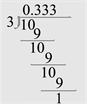. People also write this as

$\frac{1}{3}=0.3,0.33,0.333\cdots =0.\stackrel{\dot{}}{3}$ (10)

Likewise, people write.

$0.9,0.99,0.9999\cdots =0.\stackrel{\dot{}}{9}=1$ (11)

Equations Equation (10) and Equation (11) are erroneous because of using “equal sign”. The numbers 0.3, 0.33, 0.333, 0.333… are non-terminating nonlinear numbers. When 1/3 gives 0.3, there is a residue 0.1; when 1/3 gives 0.333, there is residue 0.001 etc. The 1/3 can never equate to the nonlinear numbers 0.3, 0.33, 0.333, 0.333… The fact is 1/3 is the upper asymptote of the nonlinear numbers 0.3, 0.33, 0.333, 0.333… This nonlinear numbers can approach the asymptote 1/3 but cannot touch it. The asymptote is never a part of nonlinear numbers. The 1/3 is static and the nonlinear numbers 0.3, 0.33, 0.333, 0.333… are dynamic. Static cannot equate to dynamic; we cannot violate Newton’s law.

Likewise, the numbers 0.9, 0.99, 0.999, 0.9999… are non-terminating nonlinear numbers. We need to add 0.1 to 0.9 to give 1; we need to add 0.01 to 0.99 to give 1; we need to add 0.0001 to 0.9999 to give 1 etc. The nonlinear numbers 0.9, 0.99, 0.999, 0.9999… can approach the asymptote 1, but cannot touch it. The asymptote is never a part of nonlinear numbers. The 1 is static and the nonlinear numbers 0.9, 0.99, 0.9999… are dynamic. Static cannot equate to dynamic; we cannot violate Newton’s law.

In short, we cannot use the equal sign “=” in Equation (10) and Equation (11), instead we can use an arrow → or some other sign such as ~ to relate the nonlinear numbers and the asymptote, as shown in expression (12) and (13), where each has an arrow sign. We will discuss how to measure the change (or the differential) of nonlinear numbers later.

$\frac{1}{3}=0.3,0.33,0.3333\cdots =0.\stackrel{\dot{}}{3}$ wrong

$0.3,0.33,0.333\cdots \to \frac{1}{3}$ O.K. (12)

$0.9,0.99,0.9999\cdots =0.\stackrel{\dot{}}{9}=1$ wrong

$0.9,0.99,0.9999\cdots \to 1$ O.K. (13)

The above two nonlinear numbers are regular nonlinear numbers. There are other irregular nonlinear numbers, such as $\sqrt{2}$ ~ 1.4, 1.41, 1.414, 1.4142, 1.41421, 1.414213, 1.4142135… 1.414213562… forever.

Nonlinear numbers 0.9, 0.99, 0.9999… are a one-sided nonlinear number having an upper asymptote Yu, Yu = 1. Let us compare the change of these nonlinear numbers with the change of universal linear numbers U_l and check whether the number 1 is the unique asymptote of the nonlinear numbers. Referring to Figure 12, let us input the universal linear numbers in Column A as X and the nonlinear numbers in Column B as Y, as shown in Excel Screen Figure 12.

In the Excel Screen, we reserve Cell E1 for imputing an active upper asymptote, Yu. We input 1 into Cell E1, as shown in Figure 13. We shall use this asymptote to calculate (Yu − Y) in Column C. Formula bar gives the formula for Cell C2 as “=$E$1-B2”. We then copy Cell C2 into Cell C3 through Cell C10 to complete the column. By plotting Column A vs. Column B, we obtain Figure 14(a) for X vs. Y in a linear scale, where the data line is approaching an upper asymptote, Yu. This is a primary graph and is also an asymptotic graph where the asymptotic curve is monotonically increasing and nonterminating. It is also a leading graph because the continuous changing of the slope of the curve will lead us to the proportionality relationship and equation. Now, we can visualize that the distance from asymptote Yu to Y, (Yu − Y), is negatively proportional to the linear distance of X, as shown by the solid and dashed arrow. The larger the solid arrow the smaller the dashed arrow becomes, or vise visa.

Figure 12. Nonlinear numbers 0.9, 0.99, …

Figure 13. Nonlinear numbers 0.9, 0.99, …

Refer to Figure 13, by plotting Column A vs. Column C for X vs. (Yu − Y), we obtain Figure 14(b) in linear scale; this is a pre-proportionality graph. It is also a transitional graph, because we need to convert the vertical axis into final nonlinear logarithmic scale. We can copy Figure 14(b) into Figure 14(c) and convert the vertical scale into nonlinear logarithmic scale, as shown in Figure 14(c). Notice in Figure 14(b) we are comparing (Yu − Y) vs. X in linear-by-linear scale; in Figure 14(c) we are comparing q(Yu − Y) vs. X in the log-linear scale. The next step is to display proportionality equation (trendline equation) and coefficient of determination for the proportionality plot.

Let us right click on data series in Figure 14(c) followed by selecting “Add Trendline”; and then “Exponential” from Trendline Options, also selecting “Display Trendline” and “Display R-squared”, then Close. We obtain Figure 14(d). The coefficient of determination is R² = 1. The proportionality plot of Figure 14(d) is the expression of Equation (2) and Equation (2a), with d(q(Yu − Y)) = −KdX and q(Yu − Y) = −KX + qC where K = 1 and C = 1. Ideally, the trend line equation for a straight line in a semi-log graph should be written as y = Cθ^−Kx, where C is the position constant (intercept of the straight line at X = 0) and K is the proportionality constant or the slope of the straight line. In Figure 14(d), the original equation (from using the Exponential Trendline Option) for y (=Yu − Y) vs. x is y = 1e^−2.303x; it should be written as y = 1θ^−x, where C = 1 and K = 1 (note: 2.303/2.303 = 1; 2.303 is a conversion factor between natural logarithm e and 10-based logarithm). Note: if we try to add trendline for Figure 14(c) as linear, logarithmic, polynomial, or power lines, we cannot get the desired results, as shown in Appendix A.

3) To identify the unique upper asymptote, we can use a trial-and-error or a template method

In Figure 15, let us pick a number slightly larger than 1, say, 1.0000001, and input 1.0000001 into Cell E1, as shown in Figure 15. Figure 14(d) turns into Figure 16(a), with data line strays from the straight line and R² reduced to 0.9967 (also green dots line in Figure 16(b)). When we change the number into

(a)(b)(c)(d)

Figure 14. (a) Primary graph, also a Leading Graph, Y vs. X in linear scale; (b) Pre-proportionality graph, (Yu − Y) vs. X in linear scale; (c) Proportionality graph q(Yu − Y) vs. X in log-linear scale; and (d) Proportionality graph q(Yu − Y) vs. X in log-linear scale.

Figure 15. Nonlinear numbers 0.9, 0.99, … (continued).

(a)(b)

Figure 16. (a) Proportionality graph I, q(Yu − Y) vs. X in log-linear scale, Yu = 1.0000001; (b) Proportionality graph II, q(Yu − Y) vs. X in log-linear scale, Yu = 1, 1.00001, 1.0000001, 1.0000001.

1.00001 and input 1.00001 into Cell E1, we obtain red dots line in Figure 16(b) and R² reduced to 0.9523. We can improve R² by increasing the number of zero after 1 in the numerator, such as 1.0000001. In doing this, we get yellow dots line in Figure 16(b) and the R² improves to 0.9995. The overall trend is that all the numbers eventually approach 1 as an upper asymptote. This example shows that the nonlinear numbers have an association with asymptote and that the measurement of nonlinear change needs to be measured relative to their asymptote. In short, we can express the linear relationship between linear Y and linear X using the Equation (1), while expressing the nonlinear relationship between nonlinear Y and liner X using equations Equation (2) and Equation (3). The above approach of identifying unique Yu is a trial-and-error method. We can also use a template method for general identifying of the unique asymptote as shown in Appendix C [5] [6] .

4) To handle the elusive nonlinear zero Yb, we use linear zero (0) as accessible nonlinear zero

Figure 17 lists various data for nonlinear numbers Y1 and Y2. We leave row 2 as blank for use as zero or blank in calculations. Column A (A3: A10) gives elementary numbers (x); Column B (B3: B10) gives cumulative of (x) as cumulative numbers X, where B3 = B2 + A3, B4 = B3 + A4, B5 = B4 + A5 or we can copy B3 to B4 through B10 to complete the column. Elementary numbers have no connectivity; however, the cumulative numbers have connectivity. For example, Cell A5 is 4, this 4 has no relationship with the 4 in Cell A10. On the contrary, the value in column B (B3: B10) is monotonically increasing and their values are interconnected. When we change the Cell A5 from 4 to 6, the Cell B5 changes from 8 to 10, and the Cell B10 changes from 28 into 30.

Column C (C3: C10) gives the elementary nonlinear numbers (y1), whose values may move up or down but without connectivity. Column D (D3: D10) gives cumulative of (y1) as cumulative numbers Y1, where D3 = D2 + C3, D4 = D3 + C4, D5 = D4 + C5, or we can copy D3 to D4 through D10 to complete the column. The connectivity of dependent variable Y is like that of the independent

(x) and (y) are elementary X and elementary Y, y is for equation y. X is cumulative of (x), Y is cumulative of (y).

Figure 17. Nonlinear numbers Y1 and Y2.

variable X. The elementary nonlinear numbers (y1) have no connectivity, but the cumulative nonlinear numbers Y1 have connectivity. For example, Cell C5 is 4.66, this 4.66 has no relationship with the 0.47 in Cell C10. On the contrary, the value in column D (D3: D10) is monotonically increasing and their values are interconnected. Column G (G3: G10) gives the dependent variable Y2, whose values are Y2 = 30θ^−0.5X; or Y2 − Yb = 30θ^−0.5X, with Xb = 0. These Y2 values give the asymptotic curve in Figure 3. This asymptotic cure is like that of Zeno’s nonlinear walk curve starting from the wall at 64 meter and the nonlinear equation as y = 64θ^−0.3x.

In Figure 17, Raw 12 to Raw 21 is the work area for searching the upper asymptote, Yu (see Appendix C).

By plotting Column B (B3: B10) versus Column D (D3: D10) for X versus Y1, we get the primary graph Figure 18(a), showing as an asymptotic convex curve with continuous changing of the slope. When we insert Column B (B3: B10) versus Column C (C3: C10) for X versus (y1) into Figure 18(a), we get Figure 18(b), where the elementary number curve (y1) is in the form of skewed bell. Figure 18(b) shows that it is easy to mathematically describe the asymptotic curve with equation such as Equation (2), but more difficult to describe the skewed bell with equation.

In Figure 18(a), the asymptotic curve is for the nonlinear number Y1. This Y1 has an upper asymptote Yu, as indicated with horizontal line in Figure 2 earlier. Its value is in Cell F12 of Figure 17, with Yu = 20.00. By copying Figure 18(a) and converting its vertical axis from linear into nonlinear logarithmic scale, we get Figure 19(a) along with an Excel warning banner indicating that negative or

(a)(b)

Figure 18. (a) Primary graph, cum. X vs. cum. Y, linear by linear scale; (b) Cum. X vs. cum. Y1 plus (y1), linear by linear scale.

(a)(b)(c)

Figure 19. (a) qY1 versus X in log by linear scale; (b) Y1 vs. X in linear-by-linear scale with excluding the surrogate 0; (c) Y1 in log by linear scale with excluding the surrogate 0.

zero values cannot be plotted on log scale. There are 8 data points in Figure 18(a); however, there are only 7 data points in Figure 19(a), with 6 points connected in line and with one lone point hanging outside. This is a special expression of the Excel to indicate that there is an original “surrogate zero or surrogate 0” that cannot be plotted in logarithmic scale of Figure 19(a), because this “surrogate zero, or surrogate 0” is a linear zero that cannot be plotted in a nonlinear logarithmic scale. From Figure 19(b), we can see that the asymptotic curve is a nonlinear curve for nonlinear numbers Y1. By the definition of nonlinear numbers, we should always have a bottom asymptote; and in some cases, we have both a bottom and an upper asymptote. When we plot Column B (B4: B10) versus Column D (D4: D10) for X versus Y1 with excluding the point in D3 with shaded 0.00, we get Figure 19(b) and Figure 19(c), where we get connected 7 data points in a line. The case in Figure 18(a) is that we have both a bottom and an upper asymptote. The bottom asymptote, in this case, is a nonlinear zero which cannot be expressed in a linear graph but can only be illegally represented by a “surrogate 0”.

Combination of Figures 18(a)-19(c) enhances the basic theory of alpha beta (αβ) math that the nonlinear numbers are always associated with a bottom asymptote equivalent to nonlinear zero.

Now, let us apply the face-value concept in nonlinear math to restore the 8^th data point. We know that the change of nonlinear numbers needs to measure their change relative to their asymptote. In our case, we shall need to make use of (Yu − Y1). Column E (E3: E10) gives the face-value of Y1 relative to the upper asymptote Yu. By plotting Column B (B3: B10) versus Column E (E3: E10) for X versus y, y = (Yu − Y1), we get Figure 20(a), showing as a demulative asymptotic cure. By copying Figure 20(a) and converting its vertical axis from linear into nonlinear logarithmic scale, we get the proportionality graph Figure 20(b), without trendline and coefficient of determination.

To obtain trendline equation and the coefficient of determination in the proportionality graph, we right click on data series (in Figure 20(b)). Then → adding trendline → then, in Trendline Options, select “exponential” → select “Display Equation on chart” → select “Display R-squared value on chart” → close. We obtain regression equation as y = 20e^−0.115x, and coefficient of determination R² = 1. When we select “exponential” in the Trendline Options, Excel gives us semi-log graph and provides trendline equation as exponential equation. This is awkward because Excel is not capable of providing a 10-based equation for log-linear straight line. The remedy is we convert e to θ (θ = 10) and −0.115 to −0.05 using conversion factor of 2.303 (0.115/2.303 = 0.05), as shown in Figure 20(b), where we insert y = 20θ^−0.05x.

(a)(b)

Figure 20. Face value and proportionality graph. (a) Face value graph, (Yu − Y) vs. X, linear by linear scale; (b) Proportionality graph, q(Yu − Y) vs. X, log by linear scale.

The equation y = 20θ^−kx means (Yu − Y) = Cθ^−kx. By taking log on both sides of the equation, we get q(Yu − Y) = −KX + qC, whose differential equation is d(q(Yu − Y)) = −KdX, meaning the change of nonlinear true value q(Yu − Y) is negatively proportional to the change of linear true value X, or the nonlinear change of face value (Yu − Y) is negatively proportional to the linear change of X.

Column G of Figure 17 gives a series of demulative numbers, with Cell G3 = 30.0 (at X = 0). By plotting Column B (B3: B10) versus Column G (G3: G10) for X versus Y2, we obtain Figure 21(a), showing as a concave asymptotic curve. By copying Figure 21(a) followed by converting the vertical axis from linear into nonlinear logarithmic scale, we obtain Figure 21(b) without trendline equation and coefficient of determination. We can use a similar way as Figure 20(b) to insert trendline equation and coefficient of determination R² to obtain the final Figure 20(b).

To show the characteristics of concave asymptotic curve in equation Equation (3) and Equation (3a), let us copy Figure 21(a) to get Figure 22(a) by inserting Zeno’s Series 1 and Lie Tzu’s data into the graph. We also copy Figure 21(b) to get Figure 22(b) by inserting Zeno’s Series 1 and Lie Tzu’s data into the graphs.

Figure 22(a) and Figure 22(b) illustrate the description of concave asymptotic curves for equation Equation (3) and Equation (3a). Their characteristics are: 1) the curves are associated with a bottom nonlinear asymptote; 2) the curves start at a finite value, e.g., 100, 64, and 30, equivalent to the “C” value in the trendline regression equations. The bottom nonlinear asymptotes, in general, are nonlinear zero, but they can be any numbers including a negative one [1] [4] .

(a)(b)

Figure 21. Demulative Y2 and its Proportionality graph. (a) Demulative Y2 Graph, Y2 vs. X, linear by linear scale; (b) Proportionality Graph, qY2 vs. X, log by linear scale.

(a)(b)

Figure 22. Demulative Y and their proportionality graph. (a) Demulative Y Graph, Y vs. X, linear by linear scale; (b) Proportionality Graph, qY vs. X, log by linear scale.

The “C” in Equation (3) and Equation (3a) gives the intercept of the straight-line at X = 0; the K (0.2, 0.2, and 0.05) give the slope of the straight-line. The simplest form of nonlinear equations is Equation (3) and Equation (3a) for description of concave asymptotic curves where a single bottom asymptote exists as a nonlinear zero. Equations Equation (1a), Equation (2a), and Equation (3a) are two-parameter equations where the parameter C dictates the positions of the straight-line, as shown in Figure 22(b).

The concave asymptotic curves are shown in Figure 8(a), Figure 20(a), Figure 21(a), Figure 22(a), as well as in Figure 5. In Series 1 of Figure 5, Zeno’s nonlinear walk starts from the wall of 64 meters toward the other wall of nonlinear zero. Additionally, Zeno’s Achilles in Figure 8(a) has the same meaning. In these cases, when we change the vertical axis in linear graph from linear into nonlinear logarithmic scale, we can convert the concave curve into linear straight-line in log-linear graph, such as from Figure 20(a) to Figure 20(b); Figure 21(a) to Figure 21b); Figure 22(a) to Figure 22(b); and Figure 8(a) to Figure 8(b).

Contrary to the concave asymptotic curve, the convex asymptotic curve is more troublesome and needs extra attention to its nonlinear bottom asymptote or the usage of “surrogate 0”. The convex asymptotic curve is more complicated because it involves two asymptotes: an upper asymptote and a bottom asymptote. The upper asymptote Yu can be resolved and identified through Excel operation, while the bottom asymptote is, in general, a nonlinear zero, which cannot be plotted on a linear scale or linear graph but can only be represented as Yb and calculate as a “blank cell” or “surrogate 0” in Excel operation. When we convert the vertical axis of convex asymptotic line from linear into nonlinear logarithmic scale, such as from Figure 2 or Figure 18(a) into Figure 19(a) or Figure 19(c), we don’t get a straight-line, instead we get curved lines. It is a common misconception to think that a curved line can turn into a straight-line by converting the scale from linear into logarithmic scale.

In summary, Zeno’s room-walk and Zeno’s Achille are nonlinear phenomena that can be described by the concave and convex asymptotic curves with the differential equations Equation (2) and Equation (3) along with integral equations Equation (2a) and Equation (3a). The characteristics of Equation (3a) is that there is a finite value of Y at X = 0. The characteristics of Equation (2a) is that the face-value of (Yu − Y) gives (Yu − 0) or Yu at X = 0.

5) Second order asymptotic phenomena—a phenomenon involves skewed bell and sigmoid curve

So far, we have discussed the first order asymptotic phenomena. In the real world there are more paradoxes and controversial interpretations of experiences that need to be expressed with a higher order nonlinearity of asymptotic curves, thus we shall briefly introduce and discuss the second order asymptotic phenomena in the Appendix to extend the general usage of nonlinear math.

The second order asymptotic phenomena are more varied and, to fully comprehend them, we must engage many graphs with connectivity including primitive, primary, leading, pre-proportionality (or transitional graph), and proportionality graphs. Mostly, a second order asymptotic phenomenon will involve skewed bell and sigmoidal curve. One example with discussion is given in Appendix B.

3. Summary

• The full knowledge of Zeno’s paradoxes needs to be explained in three aspects: First, need an intellectual statement; Second, need mathematical expression with αβ Math; and third, need to illustrate with graphs.

• We discussed two of Zeno’s mathematical arguments as well as Lie Tsu’s philosophy using the Alpha Beta (αβ) nonlinear math. Zeno’s room walk has three options: one linear walk and two nonlinear walks. Zeno’s Achilles has two options: one linear run and one nonlinear run. And Lie Tsu’s pole halving has one option: nonlinear halving.

• The new nonlinear concepts are the variables are classified into linear and nonlinear, and the change of a linear variable is a simple change, while the change of a nonlinear variable is a nonlinear change relative to its asymptotes. For assimilation of nonlinear experiences, we use the continuous asymptotic curves to describe and derive the equations for expressing the two-variable relationship.

• Traditional XY math is insufficient to describe the nonlinear phenomena; therefore we extend the XY math into the αβ Math to account for the existence of asymptotes, i.e., we extend XY = {(X), (Y)} into αβ = {α(Y, Yu, Yb), β(X, Xu, Xb)}.

• We can describe nonlinear phenomena with a simple proportionality equation and four types of graphs: primitive, primary, leading, and proportionality graphs. We cannot use a primitive elementary graph based on “y” to build an X-Y mathematical relationship, because each elementary “y” has no mathematical connectivity, and one elementary number cannot mathematically relate to the other cumulative numbers. Instead, we must relate one cumulative number (or demulative numbers) with another cumulative number and use the primary graph for mathematical analysis. Cumulative numbers (or demulative numbers) mean the existence of connectivity.

• In data analyses, we must always account for the origin. The peak of asymmetric bells in the primitive elementary graph depends on the size of incremental X and thus should not give any interpretation based on its height [1] [2] .

• The Alpha Beta (αβ) Math is a science for connecting a straight line to asymptotic, sigmoid, and various bell curves in biomedical and physical sciences [1] [2] . In Appendix C, we provide example for building Excel Templates to solve for upper asymptotes and building a straight-line proportionality equation using Microsoft Excel via determining the “coefficient of determination”.

• When generating regression equation for a straight line in a log-linear (semi-log) graph, we first select “exponential” option in the regression manual to get exponential equation, then followed by converting the equation into a 10-based logarithmic equation using a conversion factor of 2.303, e.g., in Figure 14(d), we convert y = 1e^−2.303X into y = 1(10)^−X, or y = 1θ^−X (see Appendix A).

• Data in science and engineering fields are mostly nonlinear and thus need to be analyzed from the viewpoint of nonlinear mathematics, where the data can be at an ordinary nonlinearity or at a higher order of nonlinearity.

• The Alpha Beta (αβ) Math is a graph-based proportion-oriented math for relating independent variable β(X, Xu, Xb) and dependent variable α(Y, Yu, Yb).

4. Conclusion

Traditional XY math is insufficient to describe the nonlinear phenomena; therefore we need to extend the XY math into the αβ Math to account for the existence of asymptotes, i.e., we extend XY = {(X), (Y)} with inclusion of X and Y into αβ = {α(Y, Yu, Yb), β(X, Xu, Xb)} with inclusion of Y, Yu, Yb, and X, Xu, Xb. Analysis of two variable relationships is best to examine their proportionality. Zeno’s paradoxes and Lie Tzu’s pole halving wisdom can be explained with first order asymptotic equations where the nonlinear change of dependent variables in term of nonlinear face-value (Y − Yb) or (Yu − Y) is proportional to the linear change of independent variable X. For the higher order of nonlinearity involving skewed bells and sigmoidal curves, we shall need to use a second order nonlinear face-value of (qYu − qY) (note: q = log).

Appendix A

Six options in Excel for expressing a straight-line data in log-linear plot.

(In Figure A1, y = 1e^−2.303x equals y = 1θ^−x, where 2.303 is a conversion factor between natural logarithm e and 10-based logarithm. Equation y = 1θ^−x means (Yu − Y) = 1θ^−x or by taking log on both sides q(Yu − Y) = q1 − X. This is q(Yu − Y) = qC − KX with C = 1, K = 1. Its differential equation is d(q(Yu − Y)) = − KdX.).

Figure A1. (a) q(Yu − Y) vs. X in log-linear scale, (b) q(Yu − Y) vs. X in log-linear scale, (c) q(Yu − Y) vs. X in log-linear scale; (d) q(Yu − Y) vs. X in log-linear scale; (e) q(Yu − Y) vs. X in log-linear scale; (f) q(Yu − Y) vs. X in log-linear scale.

Appendix B

Example of Second Order Asymptotic Phenomena [1] [5]

The second order asymptotic curve involves a convex asymptotic curve in a log-linear scale, as shown in Figure A2(c). This second order asymptotic curve originated from its primitive elementary graph in Figure A2(a) and its primary graph in Figure A2(b). In the beginning, the elementary numbers “y” gives a set of skewed bells in a linear-by-linear scale, as shown in Figure A2(a), their cumulative numbers Y give a sigmoidal curve in a linear-by-linear scale, as shown in Figure A2(b). By converting the vertical axis from linear to nonlinear logarithmic in Figure A2(b), we get a convex asymptotic curve, as shown in Figure A2(c). Figure A2(c) is a leading graph that will lead us to the pre-proportional graph in Figure A2(d) and the proportional graph in Figure A2(e).

Figure A2(c) gives the plotting of continuous nonlinear numbers Y versus linear numbers X in a log-linear scale, where the value of nonlinear variable is qY. The line starts from the origin (nonlinear zero, which is the bottom asymptote of qY and because this nonlinear zero as bottom asymptote is not part of the nonlinear numbers, it cannot be shown in the graph). Meanwhile, the curved continuous line is asymptotically approaching the upper asymptote, qYu. Again, this qYu is never a part of the qY line. The face value of this second order nonlinearity of Y is (qYu − qY). Since the change of nonlinear numbers is a nonlinear change of nonlinear face values, we need to take a nonlinear logarithmic transformation of its value to get q(qYu − qY) and designate the change of nonlinear face value as d(q(qYu − qY)). In the graph, as the solid double arrow increases, the dashed linear double arrow decreases, or vise visor. That is the solid arrows are negatively proportional to the dashed double arrows. In equation form we get equation Equation (14), indicating nonlinear change of Y in second order of nonlinearity is negatively proportional to the linear change of X, where we measure the change relative to the asymptote as (qYu − qY) and call it a second order of nonlinearity. More detailed descriptions are available in [1] [2] [3] [4] .

$d\left(q\left(qYu-qY\right)\right)=-KdX$ (14)

$q\left(qYu-qY\right)=-KX+qC$ (14a)

$d\left(q\left(qYu-qY\right)\right)=-Kd\left(q\left(X-Xb\right)\right)$ (15)

$q\left(qYu-qY\right)=-K\left(q\left(X-Xb\right)\right)+qC$ (15a)

Like the ordinary case of nonlinearity, we may have a nonlinear change of Y in second order of nonlinearity negatively proportional to a linear change of X and a nonlinear change of X. For the nonlinear-by-linear change we have Equation (14) and Equation (14a); for the nonlinear-by-nonlinear situation, we have equations Equation (15) and Equation (15a) [1] [2] [3] [4] .

Physical examples described with Equation (14) and Equation (15) are plentiful, such as the growth of soybean plants as a function of days [1] [2] or the fructose concentration versus enzyme activity [1] [2] [5] , and the percent oxygen saturation versus partial pressure of oxygen in myoglobin and hemoglobin.

(a)(b)(c)(d)(e)

Figure A2. Graphs relating to enzyme activity. (a) Primitive elementary graph y vs. X; (b) Primary graph Y vs. X; (c) Convex asymptotic graph, qY vs. X in log-linear scale; (d) Pre-proportionality graph (Yu − Y) vs. X, linear by linear scale; (e) Proportionality graph q(qYu − qY) vs. X, log by linear scale.

Appendix C

Illustration for Solving the Upper Asymptote Yu

In the following, let us use simulated data like the primary graph Figure 18(a) for illustration to obtain the upper asymptote and equation parameters using both template and trial-and-error methods.

Figure A3 illustrates a series of potential upper asymptotes Yu1 to Yu7. Our task is to identify the unique upper asymptote among them.

The following is an illustration on how to resolve for the unique optimal Yu using Microsoft Excel. First, we build a template and then systematically resolve for the Yu through solving optimal coefficient of determination R^2 (R²). The sequence is: first, select 7 to 10 estimated upper asymptotes, Yu1, Yu2, and Y3 … Yu7 (see Figure A3 Illustration A). Second, calculate the R^2 for each estimated upper asymptote, as shown in worksheet 1 to worksheet 5; and third, plot the estimated Yu vs. R^2 and visually identify the optimal Yu from the graph.

Figure A5 (Worksheet0) gives the basic data of the example. Column A gives the elementary (x); Column B is the cumulative X for succession of (x); Column C gives the elementary (y); Column D gives the cumulative Y for succession of X, e.g., D4 = D3 + C4, D5 = D4 + C5 etc. When plotting Column B vs. Column C for X versus (y), we obtain a primitive elementary graph, showing a skewed-bell curve in Figure A4(a). By plotting Column B vs. Column D for X versus cumulative Y, we obtain an asymptotic curve as shown in Figure A4(b). This is also a leading graph because it leads us to generate physical equations based on its continuous change of the slope of curve and its relationship with its upper asymptote. In the Alpha Beta (αβ) Math, the nonlinear numbers Y are associated with their asymptotes Yu and Yb. In most cases, the bottom asymptotes Yb are nonlinear zeros. Thus, we need only to solve for the upper asymptote Yu during the search for theoretical equation and parameters. Based on the new (αβ) math concept, we need to do all the calculations relative to their asymptotes. In Figure A4(b), the Y is a nonlinear number and increases from the origin toward an asymptote. However, where is the upper asymptote? How do we determine the upper asymptote?

Figure A3. Illustration A.

(a)(b)

Figure A4. Primitive elementary graph and Primary graph in linear-by-linear scales. (a) Primitive elementary graph, linear by linear scale, y vs. X; (b) Primary graph, cum. Y vs. cum. X, linear by linear scale.

(x) and (y) are elementary X and elementary Y, y is for equation y. X is cumulative of (x), Y is cumulative of (y).

Figure A5. (Worksheet 0).

In Figure A4(b), we show the upper asymptote Yu as dashed horizontal line. The graph shows that the distance of vertical solid double arrow is negatively proportional to the distance of horizontal dashed double arrow; the larger the solid double arrow the smaller the horizontal dashed double arrow becomes, or vise visa. In equation form, it is “the nonlinear change of nonlinear face-value (Yu − Y) is proportional to the linear change of linear face-value X,” or “the change of nonlinear true value q(Yu − Y) is negatively proportional to the change of linear true value X,” as shown in Equation (2). Its integral form is Equation (2a). Where K is the proportionality constant, C is an integral constant or position constant (for dictating the position of a straight-line moving up/down in a graph).

According to Equation (2a), we can plot (Yu − Y) vs. X on a log-linear graph for q(Yu − Y) vs. X to obtain a straight line when the true upper asymptote Yu is applied in the calculation. (Note: we plot nonlinear face-value (Yu − Y) on vertical logarithm scale to give true value q(Yu − Y)). To find the straight line, we first calculate y = (Yu − Y) and qy = q(Yu − Y) and plotting the equation y versus X on a log-linear (semi-log) graph. Next, let us generate a few (7 to 10) incremental estimated Yu as Yu1, Yu2, Yu3… Yu7, with initial Yu (Yu0) picked from the last largest Y number in Column D (i.e., Cell D10), Yu0 = 19.20. We assign an active incremental Yu value, ∆Yu, in Cell B12 as about one percent (1%) of Yu0, i.e., 0.02 (∆Yu = 0.02), as shown in Worksheet 1 (Figure A6). We can generate a series of estimated Yu, from Yu1 to Yu7 in Column B (B15: B21). Formula for Yu1 in Cell B15 is “=B14 + $B$12” as shown in formula bar. We copy Cell B15 to Cell B16 through Cell B21 to complete the column. By changing ∆Yu, we can obtain a wide range of estimated Yu for Yu1 to Yu7.

Next, we need to calculate Column E, Column F, and coefficient of determination R² for a given estimated Yu starting from Yu1. We assign this first Yu1 value (in Cell B15) to Cell F12, as shown in Figure A7 (Worksheet 2), and call this estimated Yu1 as key estimated active Yu (inside dashed Cell). We will use this key estimated active Yu for calculating y = (Yu − Y) in Column E, qy = q(Yu − Y) in Column F, and for calculating the Coefficient of determination R^2 in Cell F13. After the calculation, we will sequentially change the key estimated active Yu from Yu1 to Yu2, Yu3… Yu7, etc. Figure A7 (Worksheet 2) shows the calculation of Column E, the formulas bar shows the Cell E3 as “=$F$12-D3”. We copy Cell E3 to Cell E4 through Cell E10 to complete the column.

The next step is to calculate the Column F for q(Yu − Y). This is done by taking the log of Column E, e.g., the formulas bar shows the calculation of Cell F3 as “=LOG (E3)”, as shown in Figure A8 (Worksheet 3). We copy Cell F3 to Cell F4 through Cell F10 to complete the column, as shown in Worksheet 3. Next, we need to use the same key estimated active Yu in Cell F12 to calculate the Coefficient of determination R², as shown in Worksheet 4 (Figure A9). Cell F13 gives the Coefficient of Determination. There are two ways to get Coefficient of Determination. We can use either “=(CORREL (array1, array2))^2” as shown in

(x) and (y) are elementary X and elementary Y, y is for equation y. X is cumulative of (x), Y is cumulative of (y).

Figure A6. Resolving Optimal Yu (Worksheet 1).

(x) and (y) are elementary X and elementary Y, y is for equation y. X is cumulative of (x), Y is cumulative of (y).

Figure A7. (Worksheet 2).

(x) and (y) are elementary X and elementary Y, y is for equation y. X is cumulative of (x), Y is cumulative of (y).

Figure A8. (Worksheet 3).

(x) and (y) are elementary X and elementary Y, y is for equation y. X is cumulative of (x), Y is cumulative of (y).

Figure A9. (Worksheet 4).

the formula bar, or “=RSQ (known_y’s, known_x’s)”. The calculated R² can have any number of decimals, as is shown in Cell F13, where we have 0.9737884 with six decimal places.

By using 19.40 (Yu1) as key estimated active Yu in Cell F12, we obtain R^2 as 0.973788 in Cell F13. We record this number in Cell E15 (parallel to the Yu1 line) for the case of Yu1. By changing the key estimated active Yu in Cell F12 to 19.60 (Yu2), the Cell F13 changes to 0.993255. We recorded this number in Cell E16. We sequentially change the Cell F12 values from Yu2, Yu3, through Yu7 in Column B (B15: B21) and record the resulting R^2 in Cell F13 into Column E (E15: E21), as shown in Figure A10 (Worksheet 5).

For special case, when changing the key estimated active Yu in Cell F12 to 20.00 (Yu4), the Cell F13 changes to 1. We record this number in Cell E18, as shown in Figure A10 (Worksheet 5). By changing the key estimated active Yu in Cell F12 to 20.60 (Yu7), the Cell F13 changes to 0.995595. We recorded this number in Cell E21. By plotting Column B for Yu1 to Yu7 (B15: B21) versus Column E for corresponding R² in Column E (E15: E21), we obtain Figure A11, where an arrow is pointing to the optimal upper asymptote Yu, Yu = 20.00 with maximum R² at 1 is the final answer.

(x) and (y) are elementary X and elementary Y, y is for equation y. X is cumulative of (x), Y is cumulative of (y).

Figure A10. (Worksheet 5).

Figure A11. Optimal unique Yu.

The last thing to do is to express the proportionality equation and graph using the optimal upper asymptote. By assigning the optimal upper asymptote Yu (Yu = 20.00) to Cell F12, we have all data ready for graphing. We first plot Column B (B3: B10) for X vs. Column E (E3: E10) for (Yu − Y) on a linear-by-linear scale, as shown in transitional graph Figure A12(a). By converting the vertical axis from linear into nonlinear logarithmic scale in this graph, we obtain Figure A12(b) without trendline equation and without coefficient of determination. This log-linear (semi-log) graph is the proportionality graph. The transitional graph is a plot of (Yu − Y) vs. X in a linear-by-linear scale. The proportionality graph is a plot of (Yu − Y) vs. X in a log by linear scale where the true comparison is q(Yu − Y) vs. X.

To obtain trendline equation and the coefficient of determination in the proportionality graph, we right click on data series (in Figure A12(b)). Then → adding trendline → then, in Trendline Options, select “exponential” → select “Display Equation on chart” → select “Display R-squared value on chart” → close, and we obtain Figure A12(b) with regression equation as y = 20e^−0.115x, and coefficient of determination R² = 1. When we select “exponential” in the Trendline Options, Excel gives us semi-log graph and provides trendline equation as exponential equation. This is awkward because Excel is not capable of providing a 10-based equation. The remedy is to convert e to θ(θ = 10) and convert −0.115 to −0.05 using conversion factor of 2.303 (0.115/2.303 = 0.05), as shown in Figure A12(b), where y = 20θ^−0.05x. The equation y = 20θ^−kx means (Yu − Y) = Cθ^−kx . By taking log on both sides of the equation, we get q(Yu − Y) = −KX + qC, its differential equation is d(q(Yu − Y)) = -KdX, meaning the nonlinear change of nonlinear true value q(Yu − Y) is negatively proportional to the linear change of linear true value X.

Summary of the corresponding steps:

1) Use the last experimental data point as a reference upper asymptote Yu, e.g., Yu0 = 19.20) Assign an active incremental Yu value, ∆Yu , e.g., ∆Yu = 0.02 (about 1% of Yu0), such that we can generate 7 to 10 estimated upper asymptotes to cover a range of Yu, e.g., we generate estimated upper asymptotes Yu1, Yu2, Yu3… Yu7 in Column B (B14: B21); 3) Assign an estimated upper asymptote

(a) (b)

Figure A12. (a) Transitional graph, Transitional graph (Yu − Y) vs. X, Linear by linear scale and (b) Proportionality graph, q(Yu − Y) vs. X, Log by linear scale.

(e.g., Yu1) to a special Cell in Excel (e.g., Cell F12) for use to calculate nonlinear face value y = (Yu − Y) in Column E and true nonlinear values qy = log (Yu − Y) in Column F; 4) Assign a special Cell (e.g., Cell F13) for calculating coefficient of determination R^2; 5) Calculate R^2 in Cell F13 using the formula “=CORREL (B3: B10, F3: F10)^2”; 6) Copy R^2 values from Cell F13 to Cell E15 (parallel to Yu1 value); 7) Go on to the next estimated Yu (e.g., Yu2) and repeat the last 4 steps (step 3 to step 6); 8) Using the 7 estimated upper asymptotes along with its coefficient of determinations to plot estimated asymptotes versus the coefficient of determinations, (B14: B21) vs. (E14: E21), to obtain the optimal asymptote, as shown in Figure A11. The above example with Figure A11 and Figure A12 and its associated equation is like that of an example in arsenic toxicokinetic analysis presented in reference [3] .

Other than template method, we can also use the trial-and-error method: First, let us copy Figure A12(b) into Figure A13 in Excel, then high light the data area → right click the mouse → select data → click “Add” in Legend Entres → in Edit Series, enter series name Yu = 19.40 (Figure A9) → enter Column B (B3: B10) in series X values → enter Column E (E3: E10) in series Y values → OK. This is followed by adding trendline and coefficient of determination for this Yu = 19.40. Subsequently, we try out with Yu = 19.60, 20.00, and 20.60. Figure A13 indicates that only the Yu = 20.00 gives the best optimal R^2 = 1.

Attachment I

Summary of the Alpha Beta (αβ) math (an Extension of XY Math into the αβ Math)

Figure A13. Trial and error for optimal Yu, Proportionality graph, q(Yu − Y) vs. X, log by linear scale.

• We classify continuous numbers into linear and nonlinear. The key to the classification is the asymptote: liner numbers have no asymptote, such as … −3, −2, −1, 0, 1, 2, 3, 4…; In contrast, nonlinear numbers are associated with one or two asymptotes, such as …10⁻³, 10⁻², 10⁻¹, 10⁰, 10¹, 10², 10³, 10⁴…, with a nonlinear zero as bottom asymptote. The numbers decrease in steps from right to left and decrease toward nonlinear zero but will never reach or touch the nonlinear zero. Asymptote is never part of the nonlinear numbers. There are two types of zero, linear zero and nonlinear zero.

• The change of linear numbers is dY and dX. The change of nonlinear numbers is the nonlinear change relative to their asymptotes. For example, when there is one upper asymptote Yu or bottom asymptote Yb associated with Y, the nonlinear change of Y is d(q(Yu − Y)) or d(q(Y − Yb)).

• Two mathematical Axioms in the αβ Math are: Axiom I on continuity and Axiom II on asymptote.

Axiom I: Continuity exists for all collection of continuous numbers. Continuous numbers are dynamic, non-terminating, and can never be forced to stop (It is dishonest to use the uncertain word “infinity” as a disguise to stop the continuity).

Axiom II: Asymptote is approachable but cannot be touched or crossed by the continuous nonlinear numbers, i.e., asymptote is never a part of the continuous nonlinear numbers.

• The standard scale for nonlinear numbers is a 10 based logarithmic scale; its characteristic is the existence of a nonlinear zero, which is approachable but cannot be reached or touched.

• When trying to plot a zero value on a logarithmic graph using a Microsoft Excel, we will get a warning banner telling us we cannot plot a zero in the logarithmic scale. The nonlinear zero is approachable but cannot be touched and it is not plot able on the graph.

• When either the linear numbers or the cluster of nonlinear numbers are assigned or plotted on the axes of graphs, these numbers are called face values of the numbers. For linear numbers, the face values are the same as the true values. For nonlinear numbers, the face values of nonlinear numbers are not the same as the true values of nonlinear numbers. The true values of nonlinear numbers are obtained by nonlinear logarithmic transformation to the nonlinear face values. For example, when we assign a nonlinear numbers α_i to the nonlinear scale, its face-value is α_i; however, its true-value is qα_i. True-values, but not the face values, are what we need to account for when evaluating nonlinear changes. Face values of nonlinear numbers that can be assigned to the nonlinear scales may include a difference, a ratio, or a combination of both nonlinear numbers, all having nonlinear numbers measured relative to the asymptote.

Symbols

θ = 10; q = Log (nonlinear logarithmic); αβ (extension of XY); ϕ = (0) (nonlinear zero); x = elementary independent variable, y or (y) = elementary dependent variable or y = equation y (inside the graph); X = cumulative of x, Y = cumulative of y or (y).

Conflicts of Interest

The authors declare no conflicts of interest regarding the publication of this paper.

References

[1]	Hedayatkhah, A., et al. (2017) The Relationship between the Fructose Concentration and the Enzyme Activity. Universiteit Van Amsterdam, Amsterdam.
[2]	Lai, R.W., Lai, M.W., Musser, J.A. and Rehmet, P.C. (1955) The Modern Proportionality Law for Science, Medicine, and Engineering Applications. The Toshi Company, Pittsburgh, 361.
[3]	Lai, R.W. (2012) A Textbook on Nonlinearity and Proportionality in Science, Medicine, and Engineering. The Cornerstone Company, 406. (Hard Copy Book Available at http://www.lulu.com/)
[4]	Lai, R.W. (2015) The Wonderful Mathematical Connectivity of the Alpha Beta (αβ) Math. (Science of Connecting a Straight Line to Asymptotic, Sigmoid, and Various Bell Curves in Biomedical and Physical Sciences). File Posted in http://www.researchgate.net/ on 09/22/2015, V.1.
[5]	Lai, R.W., Lai, M.W. and Richardson, A.G. (1998) Unified Proportionality Equation for Modeling Biological and Pharmacological Data. Proceedings of 11th IEEE Symposium on Computer-Based Medical Systems, Lubbock, 12-14 June 1998, 104-109.
[6]	Lai, R.W. (1981) Get More Information from Flotation-Rate Data. Chemical Engineering, 181-182.