Sustainable Ecosystem Management via H_∞-Control Theory of Stochastic Systems

Michael Park

Hong Kong International School, Hong Kong, China.

DOI: 10.4236/gep.2023.112001                

Abstract

In this paper, aiming to provide accurate protocols for management of sustainable ecosystems, a design methodology of H_∞-controller for hunter-prey model under exposure to exogenous disturbance and stochastic noise is presented. Along the development, solution procedure of the stochastic Hamilton-Jacobi-Isaacs equation via Successive Galerkin’s Approximation is described. Utilizing the proposed solution methodology of Hamilton-Jacobi-Isaacs equation, H_∞-controller of hunter-prey model was successfully designed. Robustness and performance against exogenous disturbance of the designed H_∞-controller is validated and confirmed by numerical simulations including Monte-Carlo simulation by Simulink software on MATLAB.

Keywords

Galerkin Method, Feedback Design of Ecosystems, Hamilton-Jacobi Equation, Predator-Prey Model, Sustainable Ecosystem, Nonlinear Control

1. Introduction

Over the past several decades, the management of sustainable ecosystems has been an arising interest in both academia and industry Ait El Mokhtar et al. (2021), Cinner et al. (2022), Maulu et al. (2021), Mohanty et al. (2010), Rahman et al. (2022) . Typical topics include the impacts of climate change on various ecosystems including aquaculture. Management of sustainable ecosystems that can withstand such disturbances including climate change and pollution had been intensively studied in Chapin III et al. (1996) . Interactions of positive and negative feedbacks between resources and species that constrain the effects of exogenous disturbances were discussed. More researches regarding feedback of ecosystems against disturbance to environmental changes include Garnier et al. (2020), Lafuite (2017), Ortiz & Levins (2017) . Before the development of such approaches in environmental sciences, generating appropriate feedback into systems to achieve particular objectives was studied intensively on the other side of academia, the control theory.

Control theory adopts mathematical and quantitative approaches for feedback systems. Moreover, control theory had solid mathematical foundations since the past century. Hence it was validated in numerous different fields including robotics, aerospace engineering, etc. Typical objectives of control theories are the achievement of robust stability and performance against exogenous and intrinsic disturbances and noises. Although there are advantages and disadvantages among the existing control methods, optimal control theory, especially ${\mathcal{H}}_{\infty }$ -control theory provides a certain amount of margin in performance and stability of the controller. By estimating such a margin, we can predict how much modeling error and disturbance the system can withstand and maintain sustainability. It was deeply studied in van der Schaft (1992) , the ${\mathcal{H}}_{\infty }$ -control of general control-affine systems to minimize the effect of disturbances on system output. It was proved that by obtaining the smooth nonnegative solution of a certain partial differential equation (PDE), the Hamilton-Jacobi-Isaacs (HJI) equation, we can formulaically design a ${\mathcal{H}}_{\infty }$ controller of any system of the specified form.

Exploiting such advantages, there had been numerous approaches to adopt control theories outside of mechanical and aerospace engineering Del Vecchio (2016), Fiore et al. (2016), Modi et al. (2021), Shannon et al. (2020) . However, the unresolved caveat was that the systems considered were typically involved with nonlinear terms, which made HJI not solvable analytically. Such issues happened in applications in environmental engineering too.

The authors in Shastri & Diwekar (2006a, 2006b) attempted to employ optimal control theory for sustainable ecosystem management. Robustness against disturbances was the objective as other researches, but the authors explicitly derived the Pontryagin maximum principle to deduce the optimality conditions. Such approach involves numerical optimization stage of maximization of Hamiltonian, which is not tractable in general cases.

A typical method to avoid such difficulties due to nonlinearity was to find an appropriate trim point and linearize the dynamics around it. However, depending on the extent of nonlinearity, there were multiple systems that such an approach was not applicable. Moreover, whenever linearization takes place, there is no longer any guarantee available regarding the stability and performance of the controller whenever a transition between trim points occurs.

Under such background, it was proposed an iterative algorithm in Bea (1998) to solve nonlinear, deterministic Hamilton-Jacobi-Bellman (HJB) and HJI equations numerically. The methodology developed in Bea (1998) was named Successive Galerkin’s Approximation (SGA). Galerkin’s method is a method to solve a first-order PDE numerically. However, since the HJB and HJI equations were not of the first order, it was unable to adopt Galerkin’s method here. The authors in Bea (1998) applied Galerkin’s method iteratively to solve both HJB and HJI equations numerically. Moreover, the pointwise convergence property of the proposed algorithm was also proved. However since the considered equations were deterministic systems not involving any stochastic terms, the range of application was limited, especially in fields such as synthetic biology and environmental sciences.

To this end, we propose a design method of ${\mathcal{H}}_{\infty }$ -controllers of stochastic systems through modification of the SGA algorithm. The main purpose of this research can be summarized as development of formulaic design procedure of ${\mathcal{H}}_{\infty }$ controller under exogenous stochastic disturbances. However, we typically aim to apply our results to predator-prey system for the management of sustainable ecosystems due to foregoing reasons along the introduction. A modified SGA algorithm is developed and validity is confirmed through numerical simulation results on MATLAB software. This paper is organized as follows: in Section 2, ${\mathcal{H}}_{\infty }$ control problem is introduced. By modification of the iterative algorithms from Bea (1998) , the modified SGA algorithm is developed throughout Sections 3 and 4. Along Sections 5 and 6, the considered model in this paper is introduced and numerical demonstration results are depicted. Section 7 concludes the works in this paper.

2. The ${\mathcal{H}}_{\infty }$ -Control Problem

In this work, mean reverting Itô process is considered to model the predator-prey system dynamics. Let us consider a nonlinear control system as below.

$\stackrel{\dot{}}{x}\left(t\right)=f\left(x\right)+\mathcal{l}\left(x\right)u\left(x\right)+g\left(x\right)v\left(t\right)+\sigma x\stackrel{\dot{}}{W}\mathrm{,}x\left(0\right)=x_0$ (1)

where $x\in {ℝ}^n$ , $u\in {ℝ}^m$ , $v\in {ℝ}^q$ , $W\in ℝ$ for each t, and $f\mathrm{<mo>\; :\; </mo>}{ℝ}^n\mapsto {ℝ}^n$ , $\mathcal{l}\mathrm{<mo>\; :\; </mo>}{ℝ}^n\mapsto {ℝ}^{n\times m}$ , $g\mathrm{<mo>\; :\; </mo>}{ℝ}^n\mapsto {ℝ}^{n\times q}$ which are Lipschitz. $\sigma$ is the constant variance parameter and $u\left(x\right)$ denotes the state feedback. Exogenous disturbance is denoted by $v\left(t\right)$ and W is the 1-dimensional standard Wiener process. It is assumed that the system is observable through the output function $y\left(t\right)=Cx\left(t\right)$ where $C\in {ℝ}^{n\times p}$ . Under the existence of an unknown finite-energy external disturbance $v$ and stochastic noise $\stackrel{\dot{}}{W}$ entering the system, we aim to achieve robust stability and performance by a state feedback $u\left(x\right)$ . In this paper, it is assumed that $f\left(0\right)=0$ . If the system does not satisfy such assumption, state variables can be perturbed for appropriate amount as long as an equilibrium point of Equation (1) exists. (i.e. $\tilde{x}=x-x_e$ ) Now we introduce the ${\mathcal{H}}_{\infty }$ -feedback design problem throughout the remaining part of this section.

${\mathcal{H}}_{\infty }$ -Feedback Control Problem

Through ${\mathcal{H}}_{\infty }$ -feedback control, it is aimed to maintain asymptotic stability and disturbance-to-output ${\mathcal{L}}_2$ -gain under certain level $\gamma >0$ . It can be represented as below with consideration of stochastic noise.

$\frac{\mathbb{E}\left[{\displaystyle {\int }_0^{\infty }}{\Vert y\left(t\right)\Vert }^2+{\Vert u\left(x\left(t\right)\right)\Vert }_P^2\text{d}t\right]}{\mathbb{E}\left[{\displaystyle {\int }_0^{\infty }}{\Vert v\left(t\right)\Vert }_Q^2\text{d}t\right]}\le {\gamma }^2$ (2)

where $v\in {\mathcal{L}}_2\left({ℝ}^{+}\right)$ . $\Vert \cdot \Vert$ is the conventional Euclidean norm, and weighted

norms are defined as ${\Vert u\left(x\left(t\right)\right)\Vert }_Q^2=u{\left(x\left(t\right)\right)}^{\text{T}}{Q}^{-1}u\left(x\left(t\right)\right)$ and

${\Vert v\left(t\right)\Vert }_Q^2=v{\left(t\right)}^{\text{T}}{Q}^{-1}v\left(t\right)$ for $P\mathrm{,}Q\succ 0$ . In previous the studies of systems with

stochastic noise Zhang & Chen (2006) , the theorem below was proved.

Theorem 1. Consider the Hamilton-Jacobi-Isaacs (HJI) Equation below,

$\begin{array}{l}{\frac{\partial V}{\partial x}}^{\text{T}}f\left(x\right)+x^{\text{T}}{C}^{\text{T}}Cx+\frac{1}{4}{\frac{\partial V}{\partial x}}^{\text{T}}(\frac{1}{{\gamma }^2}g\left(x\right)Q^{-1}g{\left(x\right)}^{\text{T}}\\ \stackrel{}{}-\mathcal{l}\left(x\right)P^{-1}\mathcal{l}{\left(x\right)}^{\text{T}})\frac{\partial V}{\partial x}+\frac{1}{2}\sigma x^{\text{T}}\frac{{\partial }^{2}V}{\partial x^2}\sigma x=\mathrm{0,}V\left(0\right)=0\end{array}$ (3)

Suppose there exists a smooth solution $V\left(x\right)\ge 0$ satisfying the boundary condition $V\left(0\right)=0$ . Then the state feedback

$u\left(x\right)=-\frac{1}{2}{P}^{-1}\mathcal{l}{\left(x\right)}^{\text{T}}\frac{\partial V}{\partial x}$ (4)

satisfies the Ineq. (2). Moreover, the worst case disturbance is represented by

$v\left(t\right)=\frac{1}{2{\gamma }^2}{Q}^{-1}g{\left(x\right)}^{\text{T}}\frac{\partial V}{\partial x}$ (5)

The proof of the theorem above without consideration of stochastic noise was proposed and proved in Chen et al. (2008) , while it was considered here the general case with stochastic noise entering through the system dynamics. □

Remark 1. By substituting Equation (4) and Equation (5) to Equation (3), the HJI equation can be modified as

$\begin{array}{l}{\frac{\partial V}{\partial x}}^{\text{T}}\left(f\left(x\right)+\mathcal{l}\left(x\right)u\left(x\right)+g\left(x\right)v\right)+x^{\text{T}}{C}^{\text{T}}Cx\\ +{\Vert u\left(x\right)\Vert }_P^2-{\gamma }^2{\Vert v\Vert }_Q^2+\frac{1}{2}\sigma x^{\text{T}}\frac{{\partial }^{2}V}{\partial x^2}\sigma x=\mathrm{0,}V\left(0\right)=0\end{array}$ (6)

Dependency on time is omitted for sake of simplicity.

It is notable that the HJI equation above is not tractable for general nonlinear systems.

3. Iterative Solution Procedure

Throughout this section, an iterative solution procedure of the HJI equation, Equation (3), by solving sequence first order partial differential equations is depicted. Up to our knowledge, it was first proposed in Bea (1998) the numerical solution of the HJI equation in iterative form. But unlike the algorithm proposed in Bea (1998) , consideration of stochastic noise urges to modify the iteration algorithm. Let introduce the below notation for representation of partial differential equations.

Definition 1. $\begin{array}{c}\mathcal{P}\mathcal{D}\mathcal{E}\left(u\mathrm{,}v\mathrm{,}V\right)\equiv {\frac{\partial V}{\partial x}}^{\text{T}}\left(f\left(x\right)+\mathcal{l}\left(x\right)u\left(x\right)+g\left(x\right)v\right)+x^{\text{T}}{C}^{\text{T}}Cx\\ +{\Vert u\left(x\right)\Vert }_P^2-{\gamma }^2{\Vert v\Vert }_Q^2+\frac{1}{2}\sigma x^{\text{T}}\frac{{\partial }^{2}V}{\partial x^2}\sigma x\end{array}$

The partial differential equation $\mathcal{P}\mathcal{D}\mathcal{E}\left(u\mathrm{,}v\mathrm{,}V\right)=0$ with boundary condition $V\left(0\right)=0$ is equivalent to HJI Equation (3) when $u\left(x\right)$ and $v\left(t\right)$ are given as Equations (4) and (5). As $IterMax\to \infty$ , $u^{\left(IterMax\right)}\left(x\right)$ converges pointwise to the solution of Equation (6).

4. Modified Successive Galerkin Approximation

In this section, the overall implementation of Algorithm 1 is described. For the solution of $\mathcal{P}\mathcal{D}\mathcal{E}\left(u^{\left(i\right)}\mathrm{,}{v}^{\left(i\mathrm{,}j\right)}\mathrm{,}{V}^{\left(i\mathrm{,}j\right)}\right)=0$ with boundary constraint $V^{\left(i\mathrm{,}j\right)}\left(0\right)=0$ required at every iteration of Algorithm 1 is obtained by Galerkin’s Method. Galerkin’s method approximates the solution of a first order PDE with boundary constraint $V\left(0\right)=0$ with linear combination finite number of basis functions ${\left\{{\varphi }_n\right\}}_{n=1:N}$ that satisfy ${\varphi }_n\left(0\right)=0$ . The approximation is in least-square manner in Banach-space sense. Due to well founded theoretical backgrounds, Galerkin’s method is employed in various situations where numerical solutions of partial differential equations are needed Fletcher (1984) .

Exploiting Galerkin’s method to solve the inner-loop PDE in Algorithm 1 in no stochastic noise situation was proposed in Bea (1998) , so called the Successive Galerkin’s Approximation (SGA). It was also proven the pointwise convergence of the algorithm to the true solution for a complete set of functions of ${\mathcal{L}}_2$ -space. Further developing the previous conclusions, we expand the concept of SGA for solution of the HJI equation under consideration of stochastic noise throughout this section.

For a finite set of basis functions ${\left\{{\varphi }_n\right\}}_{n=1:N}$ , let $\Phi ={\left[\begin{array}{cccc}{\varphi }_1& {\varphi }_2& \cdots & {\varphi }_N\end{array}\right]}^{\text{T}}$ . Now suppose that the solution is approximated by $V\left(x\right)\approx c_1{\varphi }_1+\cdots +c_N{\varphi }_N$ . Let $c={\left[\begin{array}{cccc}{c}_1& c_2& \cdots & c_N\end{array}\right]}^{\text{T}}$ . When the set of basis functions ${\left\{{\varphi }_n\right\}}_{n=1:N}$ is given, we aim to find $c$ . Let us further denote the integration region of Galerkin method by $\Omega$ . 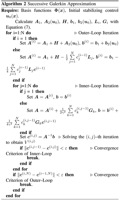The below Equation (7) are the iteration matrices for implementation of SGA. The detailed derivation in stochastic noise situation also follows the procedure at Bea (1998) .

$\begin{array}{l}{A}_1={\displaystyle {\int }_{\Omega }}F\left(x\right)f{\left(x\right)}^{\text{T}}\cdot \nabla F{\left(x\right)}^{\text{T}}\text{d}x\\ A_2\left(u_0\right)={\displaystyle {\int }_{\Omega }}F\left(x\right)u_0{\left(x\right)}^{\text{T}}\mathcal{l}{\left(x\right)}^{\text{T}}\cdot \nabla F{\left(x\right)}^{\text{T}}\text{d}x\\ b_1=-{\displaystyle {\int }_{\Omega }}{x}^{\text{T}}{C}^{\text{T}}Cx\cdot F\left(x\right)\text{d}x\\ b_2\left(u_0\right)=-{\displaystyle {\int }_{\Omega }}{\Vert u_0\left(x\right)\Vert }_P^2\cdot \Phi \left(x\right)\text{d}x\end{array}$

$\begin{array}{l}{L}_i={\displaystyle {\int }_{\Omega }}F\left(x\right){\frac{\partial {\varphi }_i}{\partial x}}^{\text{T}}\mathcal{l}\left(x\right)P^{-1}\mathcal{l}{\left(x\right)}^{\text{T}}\cdot \nabla \Phi \left(x\right)\text{d}x\mathrm{,}i=\mathrm{1,}\cdots \mathrm{,}N\\ G_i={\displaystyle {\int }_{\Omega }}F\left(x\right){\frac{\partial {\varphi }_i}{\partial x}}^{\text{T}}g\left(x\right)Q^{-1}g{\left(x\right)}^{\text{T}}\cdot \nabla \Phi \left(x\right)\text{d}x\mathrm{,}i=\mathrm{1,}\cdots \mathrm{,}N\\ H=\frac{1}{2}{\displaystyle {\int }_{\Omega }}F\left(x\right)\sigma x^{\text{T}}{\nabla }^{2}F\left(x\right)\sigma x\text{d}x\end{array}$ (7)

The vector $c^{\left(i\mathrm{,}j\right)}$ in Algorithm 2 denotes the solution of the first order PDE obtained from the previous one of $\left(i\mathrm{,}j\right)$ -th iteration, or the i-th inner loop and j-th outer loop iteration. The tolerance for termination criterion is denoted as $\epsilon$ .

5. The Predator-Prey Model

Performance of Algorithm 2 is confirmed in Predator-Prey model dynamics. Although this paper aims for design in specific Predator-Prey model, typical Predator-Prey models share analogous formulations. Hence the basis functions chosen from this paper can be adopted to the vast majority of Predator-Prey models of sustainable ecosystems. The system dynamics chosen in our research is based on Brown et al. (2005) and is given as below.

$\begin{array}{l}{\stackrel{\dot{}}{x}}_1=r_1{x}_1\left(1-\frac{x_1}{q_1}\right)+\alpha x_1{x}_2+d_1\\ {\stackrel{\dot{}}{x}}_2=r_2{x}_2\left(1-\frac{x_2}{q_2}\right)-\beta x_1{x}_2+d_2\end{array}$ (8)

where $x_1\left(t\right)$ and $x_2\left(t\right)$ denote the populations of predator and prey respectively. $d_1\left(t\right)$ and $d_2\left(t\right)$ are the external disturbance and stochastic noise term entering the dynamics. Dependency on time, t, is omitted for simplicity. The design parameters of the model including the initial conditions can be found in Table 1.

As the reference inputs are not an equilibrium point of the system dynamics, we consider the below perturbation of state and control as in Equation (9). Let $\tilde{x}=x-x_{ref}$ , $\tilde{f}\left(x\right)=f\left(x\right)-f\left(x_{ref}\right)$ , and $\tilde{u}=u+g{\left(\tilde{x}+x_{ref}\right)}^{-1}f\left(x_{ref}\right)$ .

$\begin{array}{c}\stackrel{\dot{}}{\tilde{x}}=f\left(\tilde{x}+x_{ref}\right)+g\left(\tilde{x}+x_{ref}\right)u\\ =f\left(\tilde{x}+x_{ref}\right)-f\left(x_{ref}\right)+f\left(x_{ref}\right)+g\left(\tilde{x}+x_{ref}\right)u\\ =\tilde{f}\left(\tilde{x}+x_{ref}\right)+g\left(\tilde{x}+x_{ref}\right)\left(u+g{\left(\tilde{x}+x_{ref}\right)}^{-1}f\left(x_{ref}\right)\right)\\ =\tilde{f}\left(\tilde{x}+x_{ref}\right)+g\left(\tilde{x}+x_{ref}\right)\tilde{u}\end{array}$ (9)

Table 1. Design parameters.

Note that full-state controllability is assumed in the derivation above. Now $\underset{t\to \infty }{lim}\tilde{x}\left(t\right)=\underset{t\to \infty }{lim}\tilde{u}\left(t\right)=0$ guarantees the boundedness of $V\left(x\right)$ as in Bea (1998) . By such perturbation, one can easily check that $\tilde{x}={\left[\begin{array}{cc}0& 0\end{array}\right]}^{\text{T}}$ is an equilibrium point of the system. It is noteworthy that the ${\mathcal{H}}_{\infty }$ -controller is designed with respect to the perturbed system above.

6. Numerical Demonstration & Discussion

Throughout this section, numerical demonstration results of the proposed Algorithm 2 are provided. Basis functions were chosen as $\left\{{\varphi }_1\mathrm{,}{\varphi }_2\mathrm{,}{\varphi }_3\right\}=\left\{{\tilde{x}}_1^2\mathrm{,}{\tilde{x}}_2^2\mathrm{,}{\tilde{x}}_1{\tilde{x}}_2\right\}$ . Basis functions were chosen deliberately to satisfy the property ${\varphi }_i\left(0\right)=0$ while

forming a linear approximation of $u\left(x\right)=-\frac{1}{2}{P}^{-1}\mathcal{l}{\left(x\right)}^{\text{T}}\frac{\partial V}{\partial x}$ simultaneously. Control input function was set as $g\left(x\right)=\left[\begin{array}{cc}1& 0\\ 0& 1\end{array}\right]x$ . Though Cockburn et al.

(2011) considered factors to model the success rate of hunters, as the control inputs can be scaled appropriately to compensate the failure rate, such factors were omitted in out modeling. Numerical simulations were implemented on Simulink and Matlab 2019b with Apple Macbook Pro, 2.4 GHz Intel Core i5. For the design of ${\mathcal{H}}_{\infty }$ -control, obtaining the smallest feasible value of $\gamma$ in. Equation (2) is required. Up to our knowledge, analytic solution procedure of such minimization problem is not available in nonlinear case. For linear case, with linearization of nonlinear dynamics, fuzzy interpolation approach was proposed in Chen et al. (2008) . Hence by trial and error, minimum value of $\gamma =5.3$ was set for implementation of Algorithm 2. Convergence tolerance was set as $\epsilon ={10}^{-3}$ for both inner and outer loops. It took total 7 iterations for outer loop to converge, while all the inner loop iterations converged in less than 4 iterations. Converged solution was as in Table 2.

From the obtained solution, numerical simulation was implemented on Simulink software on MATLAB. State variables and control inputs are depicted in Figure 1. During the simulation, a random seed was fed into band-limited white noise to the role as an external disturbance. $d_1$ and $d_2$ were designed to be independent random variables. The results show rapid convergence of both state and control variables to 0.

For validation of the robustness of the sustainable ecosystem designed, a Monte-Carlo simulation of total of 100 simulations was implemented. Results are shown in Figure 2, and robust stability was confirmed through the results.

Table 2. Obtained solution of the HJI with $\gamma =5.3$ .

Figure 1. Time profiles of the states and controls and disturbances.

Figure 2. Time profiles of the states, controls, and disturbances under Monte-Carlo simulation.

7. Conclusion

Throughout this paper, a sustainable management methodology of ecosystems by ${\mathcal{H}}_{\infty }$ -control theory, particularly aiming predator-prey model was developed. Modified Successive Galerkin Approximation to manage stochastic noise term was developed and employed to solve the nonlinear Hamilton-Jacobi-Isaacs equation. By numerical simulations, the robustness of the designed controller was validated.

As typical interacting systems of species in an ecosystem have similar representation, it is further expected to use the methodology presented in this paper to be applied to more general ecosystems.

Acknowledgements

I would like to express wholehearted appreciation for Hong Kong International School and my parents for supporting this research.

Conflicts of Interest

The authors declare no conflicts of interest regarding the publication of this paper.

References

[1]	Ait El Mokhtar, M., Boutasknit, A., Ben-Laouane, R., Anli, M., El Amerany, F., Salma, T., Lahbouki, S., Wahbi, S., & Abdelilah, M. (2021). Vulnerability of Oasis Agriculture to Climate Change in Morocco. In A. Karmaoui, K. Barrick, M. Reed, & M. Baig (Eds.), Impacts of Climate Change on Agriculture and Aquaculture (pp. 76-106). IGI Global. https://doi.org/10.4018/978-1-7998-3343-7.ch004
[2]	Bea, R. W. (1998). Successive Galerkin Approximation Algorithms for Nonlinear Optimal and Robust Control. International Journal of Control, 71, 717-743. https://doi.org/10.1080/002071798221542
[3]	Brown, G., Berger, B., & Ikiara, M. (2005). A Predator-Prey Model with an Application to Lake Victoria Fisheries. Marine Resource Economics, 20, 221-248. https://doi.org/10.1086/mre.20.3.42629473
[4]	Chapin III, F. S., Torn, M., & Tateno, M. (1996). Principles of Ecosystem Sustainability. American Naturalist, 148, 1016-1037. https://doi.org/10.1086/285969
[5]	Chen, B., Chang, Y.-T., & Wang, Y.-C. (2008). Robust H∞-Stabilization Design in Gene Networks under Stochastic Molecular Noises: Fuzzy-Interpolation Approach. IEEE Transactions on Systems, Man, and Cybernetics, Part B: Cybernetics, 38, 25-42. https://doi.org/10.1109/TSMCB.2007.906975
[6]	Cinner J., Caldwell, I., Thiault, L., Ben, J., Blanchard, J., Coll, M., Diedrich, A., Eddy, T., Everett, J., Folberth, C., Guiet, J., Gurney, G., Heneghan, R., Jägermeyr, J., Jiddawi, N., Lahari, R., Kuange, J., Liu, W., & Pollnac, R. (2022). Potential Impacts of Climate Change on Agriculture and Fisheries Production in 72 Tropical Coastal Communities. Nature Communications, 13, Article No. 3530. https://doi.org/10.1038/s41467-022-30991-4
[7]	Cockburn, J., McLoud, K., & Wagner, J. (2011). Robust Control of Predator-Prey-Hunter Systems. In Proceedings of the American Control Conference (pp. 1934-1939). IEEE. https://doi.org/10.1109/ACC.2011.5991093
[8]	Del Vecchio, D. (2016). Control Theory Meets Synthetic Biology. Journal of the Royal Society, Interface, 13, 20160380. https://doi.org/10.1098/rsif.2016.0380
[9]	Fiore, G., Perrino, G., di Bernardo, M., & di Bernardo, D. (2016). In Vivo Real-Time Control of Gene Expression: A Comparative Analysis of Feedback Control Strategies in Yeast. ACS Synthetic Biology, 5, 154-162. https://doi.org/10.1021/acssynbio.5b00135
[10]	Fletcher, C. A. J. (1984). Computational Galerkin Methods (1st ed.). Springer. https://doi.org/10.1007/978-3-642-85949-6_1
[11]	Garnier, A., Hulot, F., & Petchey, O. (2020). Manipulating the Strength of Organism-Environment Feedback Increases Nonlinearity and Apparent Hysteresis of Ecosystem Response to Environmental Change. Ecology and Evolution, 10, 5527-5543. https://doi.org/10.1002/ece3.6294
[12]	Lafuite, A.-S. (2017). Biodiversity Feedbacks and the Sustainability of Social-Ecological Systems. PhD Thesis, Université Toulouse III-Paul Sabatier.
[13]	Maulu, S., Hasimuna, O., Haambiya, L., Concilia, M., Musuka, C., Makorwa, T., Munganga, B., Phiri, K., & Nsekanabo, J. (2021). Climate Change Effects on Aquaculture Production: Sustainability Implications, Mitigation, and Adaptations. Frontiers in Sustainable Food Systems, 5, Article 609097. https://doi.org/10.3389/fsufs.2021.609097
[14]	Modi, S., Dey, S., & Singh, A. (2021). Noise Suppression in Stochastic Genetic Circuits Using PID Controllers. PLOS Computational Biology, 17, e1009249. https://doi.org/10.1371/journal.pcbi.1009249
[15]	Mohanty, B., Mohanty, S., Sahoo, J., & Sharma, A. (2010). Climate Change: Impacts on Fisheries and Aquaculture. In S. Simard (Ed.), Climate Change and Variability (pp. 119-138). IntechOpen. https://doi.org/10.5772/9805
[16]	Ortiz, M., & Levins, R. (2017). Self-Feedbacks Determine the Sustainability of Human Interventions in Eco-Social Complex Systems: Impacts on Biodiversity and Ecosystem Health. PLOS ONE, 12, e0176163. https://doi.org/10.1371/journal.pone.0176163
[17]	Rahman, Md., Kanon, K., Islam, Md., Mojumdar, S., Ashik, Al-A., Habibur, M., & Molla, M. H. R. (2022). Impacts of Climate Change on Aquaculture and Fisheries: An Integrated Approach for Adaptation and Mitigation. Journal of Biological Studies, 5, 10-27.
[18]	Shannon, B., Zamora-Chimal, C. G., Postiglione, L., Salzano, D., Grierson, C. S., Marucci, L., Savery, N. J., & di Bernardo, M. (2020). In Vivo Feedback Control of an Antithetic Molecular-Titration Motif in Escherichia coli Using Microfluidics. ACS Synthetic Biology, 9, 2617-2624. https://doi.org/10.1021/acssynbio.0c00105
[19]	Shastri, Y., & Diwekar, U. (2006a). Sustainable Ecosystem Management Using Optimal Control Theory: Part 1 (Deterministic Systems). Journal of Theoretical Biology, 241, 506-521. https://doi.org/10.1016/j.jtbi.2005.12.014
[20]	Shastri, Y., & Diwekar, U. (2006b). Sustainable Ecosystem Management Using Optimal Control Theory: Part 2 (Stochastic Systems). Journal of Theoretical Biology, 241, 522-532. https://doi.org/10.1016/j.jtbi.2005.12.013
[21]	van der Schaft, A. J. (1992). L2-Gain Analysis of Nonlinear Systems and Nonlinear State-Feedback H∞ Infinity Control. IEEE Transactions on Automatic Control, 37, 770-784. https://doi.org/10.1109/9.256331
[22]	Zhang, W. H., & Chen, B. (2006). State Feedback H∞ Control for a Class of Nonlinear Stochastic Systems. SIAM Journal on Control and Optimization, 44, 1973-1991. https://doi.org/10.1137/S0363012903423727