Composition of UML Class Diagrams Using Category Theory and External Constraints

Alexey Tazin, Mieczyslaw M. Kokar

Department of Electrical and Computer Engineering, Northeastern University, Boston, USA.

DOI: 10.4236/jsea.2022.1512025                

Abstract

In large software development projects, there is always a need for refactoring and optimization of the design. Usually software designs are represented using UML diagrams (e.g., class diagrams). A software engineering team may create multiple versions of class diagrams satisfying some external constraints. In some cases, subdiagrams of the developed diagrams can be selected and combined into one diagram. It is difficult to perform this task manually since the manual process is very time consuming, is prone to human errors, and is not manageable for large projects. In this paper, we present algorithmic support for automating the generation of composing diagrams, where the composed diagram satisfies a given collection of external constraints and is optimal with respect to a given objective function. The composition of diagrams is based on the colimit operation from category theory. The developed approach was verified experimentally by generating random external constraints (expressed in SPARQL and OWL), generating random class diagrams using these external constraints, generating composed diagrams that satisfy these external constraints and computing class diagram metrics for each composed diagram.

Keywords

UML, OWL, Class Diagram Composition, Reasoning, Software Requirements

1. Introduction

Refactoring plays an important role in large scale software development. Refactoring makes the design more manageable, reusable, and easy to understand by different software engineers. A software engineering team may create a class diagram based on given external constraints and then, over a period of time, create multiple refactored versions. However, the latest refactored diagram may not be optimal. In such a case, the original and all refactored versions must be reconciled. This can be achieved through creation of an optimal composed diagram using subdiagrams of given diagrams.

Diagrams may have variants in order to accommodate different customer needs. One example of this situation is Distributed Feature Composition (DFC) [1]. The development of such variants may involve multiple teams and spread across time. For maintenance purposes, it is desirable to compose such variants into a single design.

In another scenario, different teams may create diagrams modeling different parts of a system. Such diagrams may partially overlap. For integration purposes, the diagrams would have to be composed into one final diagram.

It is difficult for software engineers to achieve such reconciliation and composition of diagrams manually since the manual process is very time consuming, error prone, and not scalable for large software projects. An automated tool that can achieve this goal is desired but non-existent.

In this paper, we describe algorithms for automating the generation of a composed diagram from subdiagrams of given diagrams so that the composed diagram satisfies a given collection of external constraints and is optimal with respect to a given objective function.

It is anticipated that the process of reconciliation would be iterative, i.e., the results returned by the tool would be shown to the software engineering teams who might modify either their original diagrams or the one that is proposed by the tool and the tool would be invoked again.

In this paper, we focus on the composition of two different class diagrams based on given external constraints. The process of composition 1) selects all possible pairs of subdiagrams with given properties from two given diagrams; 2) for each pair, it computes the composition of the included subdiagrams; 3) for each composition, it computes the quality metric; 4) identifies compositions that satisfy given external constraints; and 5) selects the best composition based on the quality metrics and the objective function. The composition of subdiagrams is based on the concept of colimit from category theory.

The following correctness and quality requirements for the diagram composition method are imposed: 1) The structure and the typing of the model elements of the source (sub) diagrams with respect to the UML meta model are preserved in the composition. This is achieved by using the “correct by construction” approach (c.f. [2]), in which the ATGI-graphs are used to represent diagrams. The correctness of this approach was shown by Ehrig [3]. 2) Composition must satisfy external constraints of each of the source diagrams. This is achieved by mapping UML class diagrams to the formal language OWL (Web Ontology Language) [4] and running OWL inference using an OWL reasoner. 3) The selection of the subdiagrams and the composed class diagram must be optimal with respect to the objective function used. This is achieved by performing and exhaustive search of the subdiagrams. 4) The method of the composition should support a wide variety of class diagrams in order to be applicable in different domains. 5) Absence of redundant elements in the composed diagram [5].

The initial work on the approach described in this paper was published in [6]. The approach presented here was verified by generating random external constraints using templates, generating random UML class diagrams satisfying these external constraints, applying the composition method proposed in this paper, and assessing the quality of the solutions and performance using quantitative metrics. Moreover, we evaluated the coverage of the space of possible diagrams from which the diagrams were generated. The space was partitioned into equivalence classes, and then at least some members of each partition were tested.

Our solution to this problem is described in sections 2-4. Section 2 provides a formalization of the diagram selection optimization problem. Then section 3 shows simple examples of pairs of diagrams and composed diagrams. The algorithms for the whole solution are described in section 4. Section 5 describes the evaluation of the developed approach. Finally, section 6 presents our conclusions.

2. Optimal Diagram Construction Problem

Our problem is to develop a composed diagram using subdiagrams of two given diagrams, where the composed diagram satisfies a set of constraints and also is optimal with respect to a given objective function. In this section we provide a formalization of this optimization problem.

To formalize the optimization problem, we view UML diagrams as graphs. Assume T is a mapping from diagrams to graphs: $G=T\left(D\right)$ . Let $2^D$ be all subdiagrams of diagram D. Composition of graphs can be defined as “shared union” (more precisely—colimit) of graphs. We use symbol $\uplus$ for this operation (it is often used to represent an aggregation operation). Composition of diagrams $D_1$ and $D_2$ can be defined as composition of their graphs: $T\left(D\right)=T\left(D_1\right)\uplus T\left(D_2\right)$ . The formulation of the problem assumes that the mapping function T from diagrams to graphs is known. For composition of diagrams we reuse the same symbol as for composition of graphs. We are assuming that an objective function $f{\mathrm{<mo>\; :\; </mo>\; 2}}^D\to \mathcal{R}$ is known. This function assigns a real number to each subdiagram that represents the “quality” of a diagram.

To complete the notations we need to introduce the constraints that the diagrams must satisfy. We are assuming that a set of constraints is given as a set of expressions in a formal language. We denote such a set by $C=\left\{C_1,\cdots ,C_m\right\}$ . We also need a function that determines which subset of the constraints this subdiagram satisfies, i.e., $g{\mathrm{<mo>\; :\; </mo>\; 2}}^D\times 2^C\to Boolean$ .

Problem. Given two diagrams $G_1\mathrm{,}{G}_2$ , find a subdiagram $G_1^{\mathrm{<mo>\; *\; </mo>}}$ of $G_1$ and subdiagram $G_2^{\mathrm{<mo>\; *\; </mo>}}$ of $G_2$ , such that the composition of these subdiagrams, $G_1^{\mathrm{<mo>\; *\; </mo>}}\uplus G_2^{\mathrm{<mo>\; *\; </mo>}}$ results in the highest/lowest value of the objective function, f, provided that there exists a set of constraints $K\subset C$ that $g\left(G_1^{\mathrm{<mo>\; *\; </mo>}}\uplus G_2^{\mathrm{<mo>\; *\; </mo>}}\mathrm{,}K\right)$ is true. This statement is formalized in the following two equations.

$f\left(G_1^{\mathrm{<mo>\; *\; </mo>}}\uplus G_2^{\mathrm{<mo>\; *\; </mo>}}\right)=\underset{G_1^i\in 2^{G_1}\mathrm{,}{G}_2^j\in 2^{G_2}}{\min }f\left(G_1^i\uplus G_2^j\right)$ (1)

$\underset{K\in 2^C}{\exists }g\left(G_1^{\mathrm{<mo>\; *\; </mo>}}\uplus G_2^{\mathrm{<mo>\; *\; </mo>}}\mathrm{,}K\right)=true$ (2)

Equation (1) represents the objective function of the optimization problem. Equation (2) represents the constraints of the optimization problem.

To complete the formalization of the optimization problem we need to determine what the function g should be. In the approach presented in this paper, the determination of the satisfaction of the constraints will be achieved via mapping UML diagrams to a formal language (OWL) and representing the constraints as queries in SPARQL and then applying formal reasoning over the OWL representation of the UML class diagram and the SPARQL formulas. In this case, we use only ASK queries of SPARQL and invoke formal reasoning to derive the answer, which in this case is either TRUE of FALSE. We will use the notation $O\left(G\right)$ for the OWL representations of diagrams. The SPARQL formula representing the constraints, K, will be denoted by $O\left(K\right)$ . Additionally, we will represent the result of running an OWL inference on $O\left(G\right)$ as $O^{\mathrm{<mo>\; *\; </mo>}}\left(G\right)$ (sometimes referred to as “materialization”). Using this notation, we can rewrite Equation (2) as follows:

$O^{\mathrm{<mo>\; *\; </mo>}}\left(G_i^{\mathrm{<mo>\; *\; </mo>}}\uplus G_j^{\mathrm{<mo>\; *\; </mo>}}\right)⊢O\left(K\right)$ (3)

where “ $⊢$ ” represents the logical entailment operation. To achieve the UML to OWL mapping we use an existing tool. Similarly, the derivation is achieved by using an existing tool.

3. UML Diagram Composition Example

Figure 1(a) and Figure 1(b) show two class diagrams. These diagrams satisfy the following external constraints expressed in natural language in accordance

Figure 1. Two class diagrams.

with the semantics of associations [7] [8].

1) Every instance of class main dish is associated with at least one instance of class cook.

2) Every instance of class dessert is associated with at least one instance of class cook.

The class diagram concepts for the first external constraint are classes MainDish and Cook, and a directed association from MainDish to Cook with 1..* cardinality at the navigable end, and 0..* cardinality at the non-navigable end. The class diagram concepts for the second external constraint are classes Dessert and Cook, and a directed association from Dessert to Cook with 1..* cardinality at the navigable end, and 0..* cardinality at the non-navigable end.

The external constraints are formalized as two SPARQL ASK queries (see Listings 1 and 2) using the class diagram concepts mentioned above, based on concepts of the OWL language. The classes are declared via the rdf:type property with the value of owl:Class. The association (?p1) is declared as being of type ObjectProperty. The multiplicity is introduced through an OWL restriction, ?r1. It restricts the model to require that all instances of the classes MainDish (first example) and Dessert (second example) to be associated with at least one instance of the class Cook. This is expressed using OWL’s minQualifiedCardinality = 1 constraint applied to ?p1 using OWL’s property onProperty.

The ASK query returns true if all the clauses in the query are satisfied and false otherwise. In our approach, the satisfaction of the queries is verified by the SPARQL engine and an OWL Reasoner.

The OWL concepts used in these queries are obtained via a translation of the UML class diagrams to OWL. The queries check whether there are classes—Cook, MainDish and Dessert—that are related via a directional association from both MainDish and Dessert to Cook, whose cardinality is 1..*.

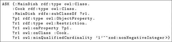
Listing 1: ASK Query 1

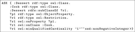
Listing 2: ASK Query 2

By visual inspection, one can see that these two queries should return true. Classes Cook, MainDish and Dessert exist in the class diagrams. The two maintained associations in Figure 1(b) play the role of p1. The relations from MainDish and Dessert to Cook in Figure 1(a) are matched to p1 through a composition of relations maintained and subClassOf.

An example of a composition of these two diagrams is shown in Figure 2. The left hand side shows two subdiagrams of the diagrams in Figure 1(b) (on the left) and Figure 1(a) (on the right). The right hand side of Figure 2 shows the composition of these two subdiagrams. The common part of these subdiagrams consists of two classes, Cook and Recipe. The composed diagram satisfies the external constraints in Listings 1 and 2. The relation from MainDish to Cook matches ?p1 of the query in Listing 1 through composition of relation maintained, relation subClassOf between MainDish and DinnerRecipe, and relation subClassOf between DinnerRecipe and Recipe. The relation from Dessert to Cook matches ?p1 of the query in Listing 2 through composition of relation maintained, relation subClassOf between Dessert and DinnerRecipe, and relation subClassOf between DinnerRecipe and Recipe. The number of classes (7) is the highest possible, the number of associations (1) is the lowest, and and the average number of ancestors (2.35) is the highest. This composition would be selected by our algorithm as optimal, based on the metrics used.

Below we show the reasoning steps a UML expert might perform on the composed diagram to see if it satisfies the first external constraint.

1. Check whether the diagram has a Cook class.

2. Check whether the diagram has a MainDish class.

3. Check whether there is a directed association from MainDish to Cook with multiplicity 1..* at the navigable end.

4. If there is no such association, check whether there is a directed association from a direct or indirect superclass of MainDish to Cook with multiplicity 1..* at the navigable end.

5. If there is no such association, check if there is a class c, directed association from c to Cook with minimum cardianality of 1 at navigable end, and directed association from MainDish to c with minimum cardianality of 1 at navigable

Figure 2. Composition of two subdiagrams.

end. The maximum cardinality at navigable end of either association should be*.

6. If there is no such class c, check if there is a class c, directed association from c to Cook with minimum cardianality of 1 at navigable end, and directed association from a direct or indirect superclass of MainDish to c with minimum cardianality of 1 at the navigable end. The maximum cardinality at the navigable end of either association should be*.

In cases 4-6, there is an implicit relation from MainDish to Cook where every instance of class MainDish is associated with at least one instance of Cook. The reasoner (by relying on general OWL axioms and ODM extension rules) will automatically infer that there is a derived association from MainDish to Cook with multiplicity 1..* at the navigable end. The query in Listing ?? will fail without this reasoning.

4. RBDC Method

In this section, we describe the basic steps of the Requirements Based Diagram Composition (RBDC) method described in this paper. It accepts two class diagrams developed in open source ArgoUML studio and a collection of external constraints expressed in SPARQL as input. The external constraints represent multiple user views of the intent of the system under development and are represented by queries against class diagrams encoded in a UML tool. The models in the tool cover both the aspects shown in the diagrams as well as the meta model of the UML. When we say that we merge UML class diagrams, we mean we merge the models that encode the class diagrams. If two elements of the diagrams have the same name, their meaning is assumed to be the same. The diagrams cannot be disconnected. Also, the input class diagram must have at least two classes with an association or generalization between them and cannot have unary associations.

The method supports the following class diagram concepts: class, generalization, binary association, association end, association end multiplicity, association end navigable property, data type (for representing primitive data types), attribute, and attribute type. The algorithmic steps of the method are listed below and then described in the subsections that follow.

1) Extract UML models from two given ArgoUML diagrams.

2) Identify all possible subdiagrams with given properties in the two UML models from the previous step.

3) Convert each subdiagram to an ATGI-graph.

4) For each pair of ATGI-graphs (one from each model), compute their shared union. The output of this step is an ATGI-graph.

5) Convert each shared union (ATGI-graph) to a UML model and an ArgoUML diagram.

6) Remove redundant attributes.

7) Convert each ArgoUML diagram to an ontology expressed in OWL.

8) Run (a) OWL inference rules using BaseVISor reasoner, and (b) ODM extension rules using SPARQL Update axioms on the ontology.

9) Identify ArgoUML diagrams that satisfy the provided set of stakeholder constraints.

10) For each diagram, compute the quality metric.

11) Select the ArgoUML diagram that has the highest value of the quality metric for the given objective function.

4.1. Extracting and Renaming UML Models

RBDC uses the ArgoUML API to extract elements of the UML model that Argo encodes. Since our objective is to merge pairs of class diagrams into one, which relies on the assumption that the elements in two diagrams with the same name actually refer to the same abstract concept, we rename the extracted elements so that this assumption is satisfied in the models. E.g., if two class diagrams have a class named Recipe, we map the extracted class elements to account for this requirement and thus the UML class ID’s of such two classes extracted through Argo will have the same ID in the translated models. This process is shown in Figure 3. In the following sections of the paper, references to a UML Model will be interpreted as references to the Renamed UML Model shown in this figure. The two mappings—Argo API and Rename—are one-to-one; they establish an equivalence relation between a UML model and the Argo model that includes the visual representation of a diagram. In the rest of the paper, we use the terms “diagram” and “model” interchageably.

A UML model is an “instance” of the UML meta model. The UML meta model is an example of an M2-model of the Meta-Object Facility (MOF) [9]. It is the model that describes the UML itself. Also, the UML meta model can be seen as a UML diagram whose instantiations are all possible UML diagrams. The meta model includes Meta- Classes, Datatypes, Attributes, Associations and Constraints. We use a simplified version of the meta model (we refer to it as the minimal UML meta model) that includes Class, Association, Property, DataType, Generalization, Element, Type and Classifier metaclasses. It is based on the meta models from [10] [11]. This version of the meta model is shown in Figure 4.

The following definition of UML model is based on [12] [13] [14]. It includes most of the elements from each of these references and adds some more.

Definition 1. A UML model of a class diagram is defined as $M=\left(C\mathrm{,}A\mathrm{,}P\mathrm{,}GEN\mathrm{,}ATTR\mathrm{,}DT\mathrm{,}Rel\right)$ , where C is a set of class symbols, A is a set of association symbols, P is a set of association end symbols, GEN is a set of generalization symbols, ATTR is a set of symbols denoting class attributes, and DT is a set of data type symbols.

Rel is a set of the mappings (listed below) of the elements of model M to either

Figure 3. Mapping UML models.

Figure 4. A Minimal UML meta model.

other elements of M or to natural numbers $\mathbb{N}$ (and −1, indicating the “*” cardinality).

· $association\mathrm{<mo>\; :\; </mo>}P\to A$

· $type\mathrm{<mo>\; :\; </mo>}ATTR\cup P\to DT\cup C$ , for $attr\in ATTR$ and $p\in P$ , $type\left(attr\right)\in DT$ and $type\left(p\right)\in C$ respectfully

· $ownedAttribute\mathrm{<mo>\; :\; </mo>}C\to 2^{ATTR\cup P}$

· $class\mathrm{<mo>\; :\; </mo>}NP\cup ATTR\to C$ , where $NP=\left\{p|p\in P\mathrm{,}\exists \mathrm{<mo>\; !\; </mo>}c\in C\mathrm{,}p\in ownedAttribute\left(c\right)\right\}$

· $memberEnd\mathrm{<mo>\; :\; </mo>}A\to 2^P$

· $ownedEnd\mathrm{<mo>\; :\; </mo>}A\to 2^P$

· $general\mathrm{<mo>\; :\; </mo>}GEN\to C$

· $specific\mathrm{<mo>\; :\; </mo>}GEN\to C$

· $lower\mathrm{<mo>\; :\; </mo>}P\cup ATTR\to \mathbb{N}$

· $upper\mathrm{<mo>\; :\; </mo>}P\cup ATTR\to \mathbb{N}\cup \left\{-1\right\}$

M must satisfy the following constraints that are applicable to the minimal meta model that we are using:

· $\forall p\in P\cup ATTR•upper\left(p\right)\ne -1\wedge lower\left(p\right)\le upper(\; p\; )$

· $\forall a\in A•\left|memberEnd\left(a\right)\right|=2$

· $ATTR\cap P=\varnothing$

· $\forall a\in A\forall p\in P•p\in memberEnd\left(a\right)\iff association\left(p\right)=a$

· $\forall g\in GEN\forall c_1\mathrm{,}{c}_2\in C•general\left(g\right)=c_1\wedge specific\left(g\right)=c_2\Rightarrow c_1\ne c_2$

· $\begin{array}{l}\forall p\in P\forall a\in A•p\in memberEnd\left(a\right)\\ \Rightarrow \left(p\in ownedEnd\left(a\right)\wedge \neg \exists c\in C•p\in ownedAttribute\left(c\right)\right)\\ \vee \left(p\notin ownedEnd\left(a\right)\wedge \exists c\in C•p\in ownedAttribute(\; c\; )\right)\end{array}$

· $\begin{array}{l}\forall p_1\mathrm{,}{p}_2\in P\forall a\in A\forall c\in C•ownedEnd\left(a\right)=\left\{p_2\right\}\wedge \left\{p_1\mathrm{,}{p}_2\right\}\\ =memberEnd\left(a\right)\wedge p_1\in ownedAttribute\left(c\right)\Rightarrow type\left(p_2\right)=c\end{array}$

· $\begin{array}{l}\forall p_1\mathrm{,}{p}_2\in NP\forall a\in A\forall c_1\mathrm{,}{c}_2\in C•\left\{p_1\mathrm{,}{p}_2\right\}=memberEnd\left(a\right)\\ \wedge p_1\in ownedAttribute\left(c_1\right)\wedge p_2\in ownedAttribute\left(c_2\right)\\ \Rightarrow type\left(p_1\right)=c_2\wedge type\left(p_2\right)=c_1\end{array}$

The Rename mapping in Figure 3 denoted here as r, is shown in Definition 2. The definition uses the function name that is implemented using the ArgoUML API. It maps every element of the model to its name. The result of the invocation of r on a UML model is a renamed model used in the processing steps that follow.

Definition 2. The renaming function r is defined in the following way:

1) $\forall c\in C•r\left(c\right)=name\left(c\right)$ .

2) $\forall dt\in DT•r\left(dt\right)=name\left(dt\right)$ .

3) $\forall attr\in ATTR•r\left(attr\right)=name\left(attr\right).name\left(class\left(attr\right)\right).name\left(type\left(attr\right)\right)$ .

4) $\forall g\in GEN•r\left(g\right)=name\left(general\left(g\right)\right).name\left(specific(\; g\; )\right)$

5) $\begin{array}{l}{\forall }_{p_1\mathrm{,}{p}_2\in P\mathrm{,}{p}_1\mathrm{,}{p}_2\in memberEnd\left(association\left(p_1\right)\right)\mathrm{,}{p}_2\ne p_1}•r\left(association\left(p_1\right)\right)\mathrm{.}\\ =name\left(association\left(p_1\right)\right)\mathrm{.}name\left(p_1\right)\mathrm{.}name\left(type\left(p_1\right)\right)\mathrm{.}lower\left(p_1\right)\mathrm{.}upper\left(p_1\right)\mathrm{.}\\ \left(p_1\in NP\right)\mathrm{.}name\left(p_2\right)\mathrm{.}name\left(type\left(p_2\right)\right)\mathrm{.}lower\left(p_2\right)\mathrm{.}upper\left(p_2\right)\mathrm{.}\left(p_2\in NP\right)\end{array}$

6) $\begin{array}{l}{\forall }_{p_1\mathrm{,}{p}_2\in P\mathrm{,}{p}_2\in ends\left(association\left(p_1\right)\right)\mathrm{,}{p}_2\ne p_1}•r\left(p_1\right)=name\left(p_1\right)\mathrm{.}name\left(type\left(p_1\right)\right)\mathrm{.}\\ lower\left(p_1\right)\mathrm{.}upper\left(p_1\right)\mathrm{.}\left(p_1\in NP\right)\mathrm{.}name\left(association\left(p_1\right)\right)\mathrm{.}name\left(p_2\right)\mathrm{.}\\ name\left(type\left(p_2\right)\right)\mathrm{.}lower\left(p_2\right)\mathrm{.}upper\left(p_2\right)\mathrm{.}\left(p_2\in NP\right)\mathrm{.}\end{array}$

4.2. Finding Subdiagrams

A subdiagram of a given model M is a diagram that includes subsets of the sets, functions that are restrictions of the functions, and constraints on M, as provided in Definition 1. This is formally captured by the following Definition 3.

Definition 3. A subdiagram of model M is defined as $M^{\prime }=\left(C^{\prime }\mathrm{,}{A}^{\prime }\mathrm{,}{P}^{\prime }\mathrm{,}GE{N}^{\prime }\mathrm{,}ATT{R}^{\prime }\mathrm{,}D{T}^{\prime }\mathrm{,}Re{l}^{\prime }\right)$ , where $C^{\prime }\subseteq C$ , $A^{\prime }\subseteq A$ , $GE{N}^{\prime }\subseteq GEN$ , $ATT{R}^{\prime }\subseteq ATTR$ and $D{T}^{\prime }\subseteq DT$ , $Re{l}^{\prime }$ is collection of restrictions of all functions from $Rel$ on $C^{\prime }$ , $A^{\prime }$ , $P^{\prime }$ , $GE{N}^{\prime }$ , $ATT{R}^{\prime }$ and $D{T}^{\prime }$ (based on [15]). Also, $M^{\prime }$ must satisfy constraints on $C^{\prime }$ , $A^{\prime }$ , $P^{\prime }$ , $GE{N}^{\prime }$ , $ATT{R}^{\prime }$ and $D{T}^{\prime }$ defined in the same way as constraints in Definition 1 by using functions from $Re{l}^{\prime }$ .

Since many subdiagrams that satisfy Definition 3 will lead to the composing diagrams unacceptable to the user or duplicate composed diagrams, our algorithm generates subdiagrams that (1) do not include disconnected classes and (2) include all the attributes of the classes.

The algorithm for finding subdiagrams is based on partitioning of $A\cup GEN$ into blocks, R, as shown in Definition 6. Generalizations are partitioned by identifying maximum connected generalization subgraphs. We do not want to break inheritance hierarchies into subdiagrams, since composition of parts of inheritance hierarchies may lead to paradoxical diagrams. The algorithm for finding inheritance hierarchies is not shown in this paper. The definitions of an inheritance hierarchy as well as sets of inheritance hierarchies of the given model are shown in Definitions 4 and 5.

Definition 4. An inheritance hierarchy in model M is $IH=\left(C_{ih}\mathrm{,}GE{N}_{ih}\right)$ , where $C_{ih}\subseteq C$ , $GE{N}_{ih}\subseteq GEN$ and for all pairs of classes $s\mathrm{,}t\in C_{ih}$ there exists a sequence of classes $s=c_0,c_1,\cdots ,c_k=t$ and $\exists g\in GE{N}_{ih}$ such that $general\left(g\right)=c_{i-1}$ and $specific\left(g\right)=c_i$ or $general\left(g\right)=c_i$ and $specific\left(g\right)=c_{i-1}$ for all $1\le i\le k$ . Also, for all $c^{\prime }\in C_{ih}$ there does not exist $g^{\prime }\in GEN\backslash GE{N}_{ih}$ such that $general\left(g^{\prime }\right)=c^{\prime }$ or $specific\left(g^{\prime }\right)=c^{\prime }$ . $I{H}_M$ is the set of all such IH for M.

Definition 5. The set of all inheritance hierarchies of model M is defined as $I{H}_M=\left\{\left(C_{ih\mathrm{,}i}\mathrm{,}GE{N}_{ih\mathrm{,}i}\right)|i\in \left\{\mathrm{1,}\cdots \mathrm{,}N\right\}\right\}$ , where $\left(C_{ih\mathrm{,}i}\mathrm{,}GE{N}_{ih\mathrm{,}i}\right)$ is an inheritance hierarchy of model M based on Definition 4 and ${\displaystyle \underset{i=1}{\overset{\left|N\right|}{\cup }}}GE{N}_{ih,i}=GEN$ . For all pairs $\left(C_{ih\mathrm{,}i}\mathrm{,}GE{N}_{ih\mathrm{,}i}\right)\mathrm{,}\left(C_{ih\mathrm{,}j}\mathrm{,}GE{N}_{ih\mathrm{,}j}\right)\in I{H}_M$ the following must be satisfied: $GE{N}_{ih,i}\cap GE{N}_{ih,j}=\varnothing$ .

Definition 6. A partition of $A\cup GEN$ is defined as $R=X\stackrel{\dot{}}{\cup }Y$ , where $X=\left\{A_i\subset A\right\}$ and $Y=\left\{GE{N}_{ih\mathrm{,}i}\subset GEN\right\}$ , $GE{N}_{ih\mathrm{,}i}$ includes generalizations of an inheritance hierarchy $I{H}_i\in I{M}_M$ , and for all pairs $A_i\mathrm{,}{A}_j\in X$ where $i\ne j$ the following must be satisfied: $A_i\cap A_j=\varnothing$ and ${{\displaystyle {\cup }_{}}}_{A_i\in X}{A}_i=A$ .

The set X used in Definition 6 is constructed in the following way. For a given integer $s<\left|A\right|$ , if $\left|A\right|mods=0$ , then A is divided into equal subsets of size s, otherwise there is also one more subset of size $\left|A\right|mods$ . The size of the blocks of the associations s is given by the user based on a desired quality of the optimal composed diagram and performance requirements. A low value of s promotes a more fine grained mix of associations from the input diagrams in the optimal composed diagram. The order in which associations are added to each $A_i$ is determined by order of associations in the implementation of A. We chose to partition associations into blocks of equal size with or without remainder.

The algorithm for finding all subdiagrams with the above properties is shown in Algorithm 1. It takes as input a model M, a partition R of $A\cup GEN$ , and outputs a set of subdiagrams, S. The following are the steps of the algorithm.

1) Find all possible subsets of blocks of R.

2) For each subset of blocks.

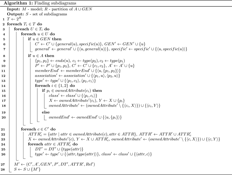
a) Find all classes connected by associations and generalizations from the subset.

b) For each identified class, find all attributes from ATTR along with datatypes from DT.

c) Create subdiagrams using associations and generalization from the subsets and identified classes, class attributes and datatypes.

The time complexity of this algorithm is $O\left(2^{m/n}\right)$ , where $m=\left|A\cup GEN\right|$ , and n is the average number of associations and generalizations per block in R. The time complexity of RBDC is discussed in Section 4.4.

4.3. Mapping UML Models to Graphs

Now we provide a formalization of the graphs that will be used to represent class diagrams. The formalization uses category theory; it is based on the work of Ehrig [3] ¹. We introduce some of the definitions to make the paper self-contained. However, some of the details are omitted. Our ultimate objective is to construct an ATGI-graph (Definition 11)—an inheritance respecting typed attributed graph, from an ArgoUML model. ATGI-graph allows to capture UML class diagram elements (e.g., classes, associations and generalizations), relations between these elements, and their properties. In addition, ATGI-graph captures types pertaining to UML class diagrams. A UML class diagram is represented using an E-graph (Definition 7). The types pertaining to the UML class diagrams come from the UML meta model which is represented as an attributed type graph with inheritance (ATGI) described in Definition 9. Considering types is important for insuring that the RBDC output—the composition of two diagrams—is a UML class diagram. The integration of an E-graph representing a UML class diagram with an ATGI representing the UML meta model is provided by a ATGI-clan morphism (Definition 10), resulting in a ATGI-graph (Definition 11).

Definition 7. (E-graph) The tuple $G=\left(V_G\mathrm{,}{V}_D\mathrm{,}{E}_G\mathrm{,}{E}_A\mathrm{,}{\left(s_j\mathrm{,}{t}_j\right)}_{j\in \left\{G\mathrm{,}A\right\}}\right)$ is an E-graph in which $V_G\mathrm{,}{V}_D$ are graph and data vertices; $E_G\mathrm{,}{E}_A$ are graph edges and node attribute edges; $s_j\mathrm{,}{t}_j$ source and target functions for graph and node attribute edges.

E-graphs will be used for representing UML models and meta-classes, meta-associations, meta-attributes and meta-datatypes of the UML meta model.

Definition 8. (UML model converted to E-graph) The graph $G_M$ is a representation of a UML model, M, as an E-graph:

$G_M=\left(V_G\mathrm{,}{V}_D\mathrm{,}{E}_G\mathrm{,}{E}_A\mathrm{,}{\left(s_j\mathrm{,}{t}_j\right)}_{j\in \left\{G\mathrm{,}A\right\}}\right)$ where:

$V_G=C\cup DT\cup GEN\cup ATTR\cup P\cup A$

$\begin{array}{l}{E}_G=\left\{\left(g,c\right)|c\in C,g\in GEN,general\left(g\right)=c\right\}\\ \stackrel{\dot{}}{\cup }\left\{\left(g,c\right)|c\in C,g\in GEN,specific\left(g\right)=c\right\}\\ \stackrel{\dot{}}{\cup }\left\{\left(c,attr\right)|c\in C,attr\in ATTR,attr\in ownedAttribute\left(c\right)\right\}\\ \stackrel{\dot{}}{\cup }\left\{\left(attr,c\right)|c\in C,attr\in ATTR,class\left(c\right)=attr\right\}\end{array}$

$\begin{array}{l}\stackrel{\dot{}}{\cup }\left\{\left(attr,dt\right)|dt\in DT,attr\in ATTR,type\left(attr\right)=dt\right\}\\ \stackrel{\dot{}}{\cup }\left\{\left(p,a\right)|p\in P,a\in A,association\left(p\right)=a\right\}\\ \stackrel{\dot{}}{\cup }\left\{\left(a,p\right)|p\in P,a\in A,p\in memberEnd\left(a\right)\right\}\\ \stackrel{\dot{}}{\cup }\left\{\left(a,p\right)|p\in P,a\in A,p\in ownedEnd\left(a\right)\right\}\end{array}$

$\begin{array}{l}\stackrel{\dot{}}{\cup }\left\{\left(p,c\right)|p\in P,c\in C,type\left(p\right)=c\right\}\\ \stackrel{\dot{}}{\cup }\left\{\left(c,p\right)|p\in P,c\in C,p\in ownedAttribute\left(c\right)\right\}\\ \stackrel{\dot{}}{\cup }\left\{\left(p,c\right)|p\in NP,c\in C,class\left(p\right)=c\right\}\end{array}$

$V_D=\left\{d|\exists p\in P\cup ATTR\mathrm{,}d=lower\left(p\right)\right\}\cup \left\{d|\exists p\in P\cup ATTR\mathrm{,}d=upper\left(p\right)\right\}$

$\begin{array}{l}{E}_A=\left\{\left(p\mathrm{,}d\right)|p\in P\cup ATTR\mathrm{,}d\in \mathbb{N}\mathrm{,}d\mathrm{<mo>\; =\; </mo>}lower\left(p\right)\right\}\\ \stackrel{\dot{}}{\cup }\left\{\left(p\mathrm{,}d\right)|p\in P\cup ATTR\mathrm{,}d\in \mathbb{N}\cup \left\{-1\right\}\mathrm{,}d=upper\left(p\right)\right\}\end{array}$

$s_G\mathrm{<mo>\; :\; </mo>}{E}_G\to V_G\equiv s_G\left(\left(s\mathrm{,}t\right)\right)=s$

$t_G\mathrm{<mo>\; :\; </mo>}{E}_G\to V_G\equiv t_G\left(\left(s\mathrm{,}t\right)\right)=t$

$s_A\mathrm{<mo>\; :\; </mo>}{E}_A\to V_G\equiv s_A\left(\left(s\mathrm{,}t\right)\right)=s$

$t_A\mathrm{<mo>\; :\; </mo>}{E}_A\to V_D\equiv t_A\left(\left(s\mathrm{,}t\right)\right)=t$

To represent inheritance in the UML meta model, we add the concept of attributed type graph with inheritance (ATGI).

Definition 9. An attributed type graph with inheritance is defined as $ATGI=\left(TG\mathrm{,}I\mathrm{,}A\right)$ where:

1) TG is an E-graph $TG=\left(T{G}_{V_G},T{G}_{V_D},T{G}_{E_G},T{G}_{E_A},{\left(s_i,t_i\right)}_{i\in \left\{G,A\right\}}\right)$ that represents the meta-classes, meta-associations, meta-attributes and meta-datatypes of the UML meta model.

2) Inheritance graph $I=\left(I_V\mathrm{,}{I}_E\mathrm{,}s\mathrm{,}t\right)$ representing the inheritance structure of the meta model, with $I_V=T{G}_{V_G}$ , $I_E$ —the inheritance edges, and the source and target functions $s\mathrm{,}t\mathrm{<mo>\; :\; </mo>}{I}_E\to I_V$

3) A set $A\subseteq I_V$ representing the abstract nodes that are involved in the inheritance relation

4) For each node $n\in I_V$ the inheritance clan is defined as $cla{n}_I\left(n\right)\mathrm{<mo\; stretchy="false">\; )\; </mo>}=\{n^{\prime }\in I_V|\exists$ path from $n^{\prime }$ to n in $I\}\subseteq I_V$ with $n\in cla{n}_I\left(n\right)$ .

The graphs representing the UML meta model and a model are combined via the mapping that is defined by an ATGI-clan morphism.

Definition 10. (ATGI-clan morphism) An ATGI clan morphism, $typ{e}_G$ , is defined as the mapping between $G_M$ representing a UML model, M, and ATGI representing the UML meta model:

$typ{e}_G\mathrm{<mo>\; :\; </mo>}{G}_M\to ATGI$ with $typ{e}_G=\left(typ{e}_{V_G}\mathrm{,}typ{e}_{V_D}\mathrm{,}typ{e}_{E_G}\mathrm{,}typ{e}_{E_A}\right)$ , where:

1. $typ{e}_{V_G}:V_G\to T{G}_{V_G}$

2. $typ{e}_{V_D}:V_D\to T{G}_{V_D}$

3. $typ{e}_{E_G}:E_G\to T{G}_{E_G}$

4. $typ{e}_{E_A}:E_A\to T{G}_{E_A}$

and $typ{e}_G$ commutes with sources and targets of $G_M$ as well as sources, targets and inheritance clan of ATGI as detailed in [3].

$typ{e}_{V_G}$ , $typ{e}_{V_D}$ , $typ{e}_{E_G}$ , $typ{e}_{E_A}$ are defined follows:

1. $typ{e}_{V_G}\left(v\right)=Class$ , where $v\in C$ .

2. $typ{e}_{V_G}\left(v\right)=Property$ , where $v\in P\cup ATTR$ .

3. $typ{e}_{V_G}\left(v\right)=Association$ , where $v\in A$ .

4. $typ{e}_{V_G}\left(v\right)=Generalization$ , where $v\in GEN$ .

5. $typ{e}_{V_G}\left(v\right)=Datatype$ , where $v\in DT$ .

6. $typ{e}_{E_G}\left(\left(g,c\right)\right)=general$ , where $g\in GEN$ , $c\in C$ and $general\left(g\right)=c$ .

7. $typ{e}_{E_G}\left(\left(g,c\right)\right)=specific$ , where $g\in GEN$ , $c\in C$ and $specific\left(g\right)=c$ .

8. $typ{e}_{E_G}\left(\left(c\mathrm{,}attr\right)\right)=ownedAttribute$ , where $c\in C$ , $attr\in ATTR$ and $attr\in ownedAttribute\left(c\right)$ .

9. $typ{e}_{E_G}\left(\left(attr\mathrm{,}c\right)\right)=class$ , where $c\in C$ , $attr\in ATTR$ and $class\left(c\right)=attr$ .

10. $typ{e}_{E_G}\left(\left(attr\mathrm{,}dt\right)\right)=type$ , where $dt\in DT$ , $attr\in ATTR$ and $type\left(attr\right)=dt$ .

11. $typ{e}_{E_G}\left(\left(p\mathrm{,}a\right)\right)=association$ , where $p\in P$ , $a\in A$ and $association\left(p\right)=a$ .

12. $typ{e}_{E_G}\left(\left(a\mathrm{,}p\right)\right)=memberEnd$ , where $p\in P$ , $a\in A$ and $p\in memberEnd\left(a\right)$ .

13. $typ{e}_{E_G}\left(\left(a\mathrm{,}p\right)\right)=ownedEnd$ , where $p\in P$ , $a\in A$ and $p\in ownedEnd\left(a\right)$ .

14. $typ{e}_{E_G}\left(\left(p\mathrm{,}c\right)\right)=type$ , where $p\in P$ , $c\in C$ and $type\left(p\right)=c$ .

15. $typ{e}_{E_G}\left(\left(c\mathrm{,}p\right)\right)=ownedAttribute$ , where $p\in P$ , $c\in C$ and $p\in ownedAttribute\left(c\right)$ .

16. $typ{e}_{E_G}\left(\left(p\mathrm{,}c\right)\right)=class$ , where $p\in NP$ , $c\in C$ and $class\left(p\right)=c$ .

17. $typ{e}_{V_D}\left(d\right)=Integer$ , where $\exists p\in P\cup ATTR•d=lower\left(p\right)\vee d=upper\left(p\right)$ .

18. $typ{e}_{E_A}\left(\left(p\mathrm{,}d\right)\right)=lower$ , where $p\in P\cup ATTR$ , $d\in \mathbb{N}$ and $d=lower\left(p\right)$ .

19. $typ{e}_{E_A}\left(\left(p\mathrm{,}d\right)\right)=upper$ , where $p\in P\cup ATTR$ , $d\in \mathbb{N}\cup \left\{-1\right\}$ and $d=upper\left(p\right)$ .

Definition 11. (ATGI-graph) Given an E-graph G representing a UML class diagram, an attributed type graph ATGI with inheritance that represents the UML meta model, and an ATGI-clan morphism $typ{e}_G\mathrm{<mo>\; :\; </mo>}G\to ATGI$ representing the typing of the class diagram by the meta model; then $G^I=\left(G\mathrm{,}typ{e}_G\right)$ is an inheritance respecting typed attributed graph (ATGI-graph).

Figure 5 shows a graphical representation of the ATGI that captures the meta model shown in Figure 4. TG and I of the meta model ATGI are merged into one graph, where the edges of I are shown using hollow arrows. This notation was borrowed from [3].

Figure 6 shows an example of a correspondence between an ATGI-graph and a UML class diagram using a graphical representation used by Ehrig in [3] in

Figure 5. ATGI representing the UML minimal meta model.

Figure 6. Mapping between a class diagram (bottom) and an ATGI-graph (top).

which the class diagram is shown at the bottom and an ATGI-graph at the top. The boxes of the ATGI-graph are elements of $V_G$ , the arrows between the boxes are elements of $E_G$ . The data nodes (elements of $V_D$ ) of the E-graph are shown as values of attributes in the boxes (e.g., upper: −1 represents an $E_A$ ). The types of the graph vertices, $V_G$ , are shown using the UML-like notation for classes (e.g., p1: Property). For the graph edges, $E_G$ , and node attribute edges, $E_A$ , only the types are shown. For the data vertices, $V_D$ , types are omitted.

The blue arrows show (partially) mapping from the elements of the class diagram to the nodes of the ATGI-graph. Meta-associations between elements of the class diagram are mapped to the associations. Meta-attributes of the class diagram elements are mapped to the elements of $E_A$ and values of meta-attributes are mapped to elements of $V_D$ , e.g., the upper bound of the multiplicity [*] goes to upper: −1.

The names of the elements of $E_G$ are computed by concatenating the names of the sources and targets, and their types. The names of the elements of $E_A$ are computed by concatenating the names of the sources, values of the targets, and their types.

4.4. Shared Unions of Pairs of ATGI-Graphs

The process of computing a shared union is depicted in Figure 7. The input to the process is a pair of ATGI-graphs $G_1^I=\left(G_1\mathrm{,}typ{e}_{G_1}\right)$ and $G_2^I=\left(G_2\mathrm{,}typ{e}_{G_2}\right)$ , where $G_i=\left(G_{i\mathrm{,}{V}_G}\mathrm{,}{G}_{i\mathrm{,}{V}_D}\mathrm{,}{G}_{i\mathrm{,}{E}_G}\mathrm{,}{G}_{i\mathrm{,}{E}_A}\mathrm{,}{\left(s_{G_{i\mathrm{,}j}}\mathrm{,}{t}_{G_{i\mathrm{,}j}}\right)}_{j\in \left\{G\mathrm{,}A\right\}}\right)$ and $typ{e}_{G_i}\mathrm{<mo>\; :\; </mo>}{G}_i\to ATGI$ for $i=1,2$ . ATGI is defined in Definition 9; it represents a UML meta model

Figure 7. Construction of shared union.

shown in Figure 5. The output is an ATGI-graph $G_3^I=\left(G_3\mathrm{,}typ{e}_{G_3}\right)$ representing a shared union of $G_1^I$ and $G_2^I$ , where $typ{e}_{G_3}\mathrm{<mo>\; :\; </mo>}{G}_3\to ATGI$ . The following are the steps of the process.

1. Step 1: Construct the disjoint unions of the components ( $V_G$ , $E_G$ , $V_D$ , $E_A$ ) of $G_1$ and $G_2$ listed in Definition 8.

2. Step 2: Define equivalence relations on the disjoint unions from the previous step and insert elements of the disjoint unions to $G_3$ where equivalent elements are glued together.

3. Step 3: Construct injective E-graph morphisms $f\mathrm{<mo>\; :\; </mo>}{G}_1\to G_3$ , $g\mathrm{<mo>\; :\; </mo>}{G}_2\to G_3$ using the equivalence relations defined in the previous step.

4. Step 4: Compute an E-graph $G_4$ (the largest common subgraph of $G_1$ and $G_2$ ) and E-graph morphisms $f^{\prime }\mathrm{<mo>\; :\; </mo>}{G}_4\to G_1$ , $g^{\prime }\mathrm{<mo>\; :\; </mo>}{G}_4\to G_2$ as pullback using $G_1$ , $G_2$ , $G_3$ , f and g.

5. Step 5: Compute $G_3^I=\left(G_3,typ{e}_{G_3}\right)$ using $typ{e}_{G_1}$ , $typ{e}_{G_2}$ and pushout $\left(G_3\mathrm{,}f\mathrm{,}g\right)$ .

Below, we present descriptions of the steps, starting with Step 2.

Step 2: Equivalence relations on disjoint unions of components of $G_1$ and $G_2$ are computed on the assumption of uniqueness of names, i.e., elements that have the same names are glued into one equivalence class in $G_3$ .

1. $\left[v\right]=\left\{v^{\prime }\in G_{\mathrm{1,}{V}_G}\stackrel{\dot{}}{\cup }{G}_{\mathrm{2,}{V}_G}\mathrm{<mo>\; |\; </mo>}{v}^{\prime }=v\right\}$ .

2. $\left[e\right]=\left\{e^{\prime }\in G_{\mathrm{1,}{E}_G}\stackrel{\dot{}}{\cup }{G}_{\mathrm{2,}{E}_G}\mathrm{<mo>\; |\; </mo>}{e}^{\prime }=e\wedge s_G\left(e^{\prime }\right)=s_G\left(e\right)\wedge t_G\left(e^{\prime }\right)=t_G\left(e\right)\right\}$ .

3. $\left[d\right]=\left\{d^{\prime }\in G_{1,V_D}\stackrel{\dot{}}{\cup }{G}_{2,V_D}|d^{\prime }=d\right\}$ .

4. $\left[a\right]=\left\{a^{\prime }\in G_{1,E_A}\stackrel{\dot{}}{\cup }{G}_{2,E_A}|a^{\prime }=a\wedge s_A\left(a^{\prime }\right)=s_A\left(a\right)\wedge t_A\left(a^{\prime }\right)=t_A\left(a\right)\right\}$ .

5. $s_{G_{\mathrm{3,}G}}\mathrm{<mo>\; :\; </mo>}{G}_{\mathrm{3,}{E}_G}\to G_{\mathrm{3,}{V}_G}\equiv s_{G_{\mathrm{3,}G}}\left(\left[e\right]\right)=\left[s_G\left(e\right)\right]$ .

6. $t_{G_{3,G}}:G_{3,E_G}\to G_{3,V_G}\equiv t_{G_{3,G}}\left(\left[e\right]\right)=\left[t_G\left(e\right)\right]$ .

7. $s_{G_{3,A}}:G_{3,E_A}\to G_{3,V_G}\equiv s_{G_{3,A}}\left(\left[a\right]\right)=\left[s_A\left(a\right)\right]$ .

8. $t_{G_{3,A}}:G_{3,E_A}\to G_{3,V_D}\equiv t_{G_{3,A}}\left(\left[a\right]\right)=\left[t_A\left(a\right)\right]$ .

Step 3: The morphisms $f\mathrm{<mo>\; :\; </mo>}{G}_1\to G_3$ , $g\mathrm{<mo>\; :\; </mo>}{G}_2\to G_3$ are computed component-wise: $f=\left(f_{V_G}\mathrm{,}{f}_{E_G}\mathrm{,}{f}_{V_D}\mathrm{,}{f}_{E_A}\right)$ , $g=\left(g_{V_G}\mathrm{,}{g}_{E_G}\mathrm{,}{g}_{V_D}\mathrm{,}{g}_{E_A}\right)$ .

1. $f_{V_G}\left(v\right)=\left[v\right],g_{V_G}\left(v\right)=\left[v\right]$ .

2. $f_{E_G}\left(e\right)=\left[e\right],g_{E_G}\left(e\right)=\left[e\right]$ .

3. $f_{V_D}\left(d\right)=\left[d\right],g_{V_D}\left(d\right)=\left[d\right]$ .

4. $f_{E_A}\left(a\right)=\left[a\right],g_{E_A}\left(a\right)=\left[a\right]$ .

Step 4: $G_4$ and morphisms $f^{\prime }\mathrm{<mo>\; :\; </mo>}{G}_4\to G_1$ , $g^{\prime }\mathrm{<mo>\; :\; </mo>}{G}_4\to G_2$ are computed component-wise using the algorithm for the pullback for attributed graphs [17].

1. $G_{4,V_G}=\left\{\left(v_1,v_2\right)\in G_{1,V_G}\times G_{2,V_G}|f_{V_G}\left(v_1\right)=g_{V_G}\left(v_2\right)\right\}$ .

2. $G_{4,E_G}=\left\{\left(e_1,e_2\right)\in G_{1,E_G}\times G_{2,E_G}|f_{E_G}\left(e_1\right)=g_{E_G}\left(e_2\right)\right\}$ .

3. $G_{4,V_D}=\left\{\left(d_1,d_2\right)\in G_{1,V_D}\times G_{2,V_D}|f_{V_D}\left(d_1\right)=g_{V_D}\left(d_2\right)\right\}$ .

4. $G_{4,E_A}=\left\{\left(a_1,a_2\right)\in G_{1,E_A}\times G_{2,E_A}|f_{E_A}\left(a_1\right)=g_{E_A}\left(a_2\right)\right\}$ .

Source and target functions for $G_4$ are determined in the following way.

1. $s_{G_{4,G}}:G_{4,E_G}\to G_{4,V_G}\equiv s_{G_{4,G}}\left(\left(e_1,e_2\right)\right)=\left(s_{G_{1,G}}\left(e_1\right),s_{G_{2,G}}\left(e_2\right)\right)$ .

2. $t_{G_{4,G}}:G_{4,E_G}\to G_{4,V_G}\equiv t_{G_{4,G}}\left(\left(e_1,e_2\right)\right)=\left(t_{G_{1,G}}\left(e_1\right),t_{G_{2,G}}\left(e_2\right)\right)$ .

3. $s_{G_{4,A}}:G_{4,E_A}\to G_{4,V_G}\equiv s_{G_{4,A}}\left(\left(a_1,a_2\right)\right)=\left(s_{G_{1,A}}\left(a_1\right),s_{G_{2,A}}\left(a_2\right)\right)$ .

4. $t_{G_{4,A}}:G_{4,E_A}\to G_{4,V_D}\equiv t_{G_{4,A}}\left(\left(a_1,a_2\right)\right)=\left(t_{G_{1,A}}\left(a_1\right),t_{G_{2,A}}\left(a_2\right)\right)$ .

The morphisms $f^{\prime }$ , $g^{\prime }$ are computed component-wise as shown below. It is easy to show that the morphisms commute: $f\circ f^{\prime }=g\circ g^{\prime }$ , as required by the definition of pullback.

1. ${f^{\prime }}_{V_G}\left(\left(v_1,v_2\right)\right)=v_1$ , ${g^{\prime }}_{V_G}\left(\left(v_1,v_2\right)\right)=v_2$ .

2. ${f^{\prime }}_{E_G}\left(\left(e_1,e_2\right)\right)=e_1$ , ${g^{\prime }}_{E_G}\left(\left(e_1,e_2\right)\right)=e_2$ .

3. ${f^{\prime }}_{V_D}\left(\left(d_1,d_2\right)\right)=d_1$ , ${g^{\prime }}_{V_D}\left(\left(d_1,d_2\right)\right)=d_2$ .

4. ${f^{\prime }}_{E_A}\left(\left(a_1,a_2\right)\right)=a_1$ , ${g^{\prime }}_{E_A}\left(\left(a_1,a_2\right)\right)=a_2$ .

Step 5: To complete the construction of $G_3^I$ , the morphism $typ{e}_{G_3}\mathrm{<mo>\; :\; </mo>}{G}_3\to ATGI$ is computed using $typ{e}_{G_1}\mathrm{<mo>\; :\; </mo>}{G}_1\to ATGI$ , $typ{e}_{G_2}\mathrm{<mo>\; :\; </mo>}{G}_2\to ATGI$ and pushout $\left(G_3\mathrm{,}f\mathrm{,}g\right)$ based on pushout property of ATGI-clan morphisms from [17], where $typ{e}_{G_3}\circ f=typ{e}_{G_1}$ and $typ{e}_{G_3}\circ g=typ{e}_{G_2}$ . $\left(G_3\mathrm{,}f\mathrm{,}g\right)$ is pushout according to relationship between pushout and pullback described in [17], since $\left(G_4\mathrm{,}{f}^{\prime }\mathrm{,}{g}^{\prime }\right)$ is pullback. The morphism $typ{e}_{G_3}$ is computed component-wise: $typ{e}_{G_3}=\left(typ{e}_{G_3\mathrm{,}{V}_G}\mathrm{,}typ{e}_{G_3\mathrm{,}{E}_G}\mathrm{,}typ{e}_{G_3\mathrm{,}{V}_D}\mathrm{,}typ{e}_{G_3\mathrm{,}{E}_A}\right)$ .

1. $typ{e}_{G_3,V_G}\left(f_{V_G}\left(v\right)\right)=typ{e}_{G_1,V_G}\left(v\right)$ , $typ{e}_{G_3,V_G}\left(g_{V_G}\left(v\right)\right)=typ{e}_{G_2,V_G}\left(v\right)$ .

2. $typ{e}_{G_3,E_G}\left(f_{E_G}\left(e\right)\right)=typ{e}_{G_1,E_G}\left(e\right)$ , $typ{e}_{G_3,E_G}\left(g_{E_G}\left(e\right)\right)=typ{e}_{G_2,E_G}\left(e\right)$ .

3. $typ{e}_{G_3,V_D}\left(f_{V_D}\left(d\right)\right)=typ{e}_{G_1,V_D}\left(d\right)$ , $typ{e}_{G_3,V_D}\left(g_{V_D}\left(d\right)\right)=typ{e}_{G_2,V_D}\left(d\right)$ .

4. $typ{e}_{G_3,E_A}\left(f_{E_A}\left(a\right)\right)=typ{e}_{G_1,E_A}\left(a\right)$ , $typ{e}_{G_3,E_A}\left(g_{E_A}\left(a\right)\right)=typ{e}_{G_2,E_A}\left(a\right)$ .

The time complexity of the algorithm for constructing shared unions of pairs of diagrams is as follows. Assume that $D_1$ and $D_2$ are two input diagrams, $A_1$ and $GE{N}_1$ are associations and generalizations of $D_1$ , and $A_2$ and $GE{N}_2$ are associations and generalizations of $D_2$ . The time complexity of the algorithm is $O\left(2^{\left(m_1+m_2\right)/n}\right)$ , where $m_1=\left|A_1\cup GE{N}_1\right|$ and $m_2=\left|A_2\cup GE{N}_2\right|$ .

In fact, this represents the time complexity of RBDC. Also, the time complexity of RBDC is further reduced by generating shared unions that are connected graphs. The performance of RBDC is in Section 5.3 describing the results of our evaluation.

4.5. Removing Redundant Attributes

The composed UML model resulting from the algorithms described above may contain some redundancies, e.g., the same attribute appearing in both sub and superclasses. The redundancies addressed in our algorithms are captured in the following definition.

Definition 12. Class $c_{super}\in C$ is a superclass class of class $c\in C$ if $s_{super}\ne c$ and there exists a sequence of classes $c_{super}=c_0\mathrm{,}{c}_1\mathrm{,}\cdots ,c_k=c$ and $\exists g\in GEN$ such that $general\left(g\right)=c_{i-1}$ and $specific\left(g\right)=c_i$ for all $1\le i\le k$ .

The algorithm does the following. If the class $c\in C$ of model M has an attribute $attr\in ATTR$ (along with datatype $dt\in DT$ ), and there is a superclass of c that has attribute $att{r}^{\prime }\in ATTR$ (along with datatype $d{t}^{\prime }\in DT$ ), where $name\left(att{r}^{\prime }\right)=name\left(attr\right)$ and $d{t}^{\prime }=dt$ , then remove attr from ATTR, $\langle c\mathrm{,}attr\rangle$ from owned Attribute, $\langle attr\mathrm{,}dt\rangle$ from type and $\langle attr\mathrm{,}c\rangle$ from class.

4.6. Representing UML Class Diagrams in OWL

The conversion of UML class diagrams to OWL is based on the Ontology Definition Meta model (ODM) specification [18] that describes the mapping between UML elements and OWL entities. The mapping is achieved using an existing tool—UML2OWL, by Leinhos—described in [19]. The original tool supports reading class diagrams in XMI 1.2 format implemented by Poseidon 4.1. We modified the tool to allow support of class diagrams in XMI 1.2 format implemented by ArgoUML. Also, we added support of property qualified cardinality restrictions.

4.7. Running OWL and ODM Extension Rules

Some of the assertions that are needed to infer that the external constraints are satisfied may not be explicit in the diagram ontology initially but can be inferred based on class diagram elements that are explicit. Examples of such implicit assertions supported by RBDC are statements about derived associations (including those that are based on inherited association ends), chains of generalizations, and inherited class attributes.

Derived associations based on inherited association ends, chains of generalizations and inherited class attributes are inferred using the axiom of the transitivity of the subClassOf property. The axiom is executed by BaseVISor (OWL2 RL) reasoner [20].

The inference of other kinds of derived associations are not supported by the rules obtained through the ODM mapping of UML to OWL. Therefore, we had to extend the mapping using SPARQL Update query [21] axioms. The SPARQL Update query axioms are based on the rules of class diagram abstraction studied in the thesis [22]. The following is a representation of the axioms in UML terms.

In this notation, A, B, and C represent classes, hollow arrows represent generalizations, lines represent bidirectional associations, regular arrows represent directed associations. Labels on the lines and arrows represent multiplicities. The left hand side of each axiom corresponds to the query’s WHERE clause—a conjunction of the triples for matching the representations of the corresponding class diagram elements in the diagram’s ontology. The right hand side of each axiom corresponds to the query’s INSERT clause—a conjunction of the triples specifying inferred and asserted object properties and property restrictions representing derived associations.

4.8. Computation of Diagram Quality Metrics and Selection of Optimal Solutions

The objective function for the optimization is based on the following software metrics of the composed diagrams: 1) the number of classes (NC), 2) the number of associations (NA), 3) the number of inheritance hierarchies (NIH), 4) attribute inheritance factor (AIF)—this is the ratio of the number of inherited attributes to the total number of attributes in a diagram, 5) average number of ancestors (ANA), 6) the number of generalizations (NG). These metrics impact the design quality attributes studied in [23] that are related to the class diagram concepts supported by RBDC. Specifically, they impact the following design quality attributes: reusability, understandability, functionality, effectiveness, extendibity, and design simplicity. Following [23] [24] [25] and [26], an increase of the metric increases (↑) or decreases (↓) the quality attributes, as shown in Table 1.

Table 1. Relationship between quality metrics and design attributes.

Our problem is a Multi-Objective Optimization Problem (MOOP). Our implementation of the solution relies on the global criterion method described in [27] and is classified as a no-preference method. We considered six objective functions that measure specific design qualities. In the cases where more than one metric influences the quality attribute, the contributing metrics are added together using the same weights. This choice is totally arbitrary; however the designers who might want to use RBDC could set their own preferred weights.

1. Reusability: $f_1=\frac{1}{2}\left(NC+AIF\right)$ .

2. Understandability: $f_2=-\frac{1}{3}\left(NC+AIF+ANA\right)$ .

3. Functionality: $f_3=\frac{1}{2}\left(NIH+NC\right)$ .

4. Effectiveness: $f_4=ANA$ .

5. Extedibility: $f_5=ANA$ .

6. Simplicity: $f_6=-\frac{1}{4}\left(NA+AIF+NIH+NG\right)$ .

The MOOP objective function is $f={\left[f_1\mathrm{,}{f}_2\mathrm{,}{f}_3\mathrm{,}{f}_4\mathrm{,}{f}_5\mathrm{,}{f}_6\right]}^{\text{T}}$ . Since this was a minimization problem, the inverses of all the objective functions were minimized. The ideal point, $z^{ideal}$ , is obtained by finding the minimum value for each objective function separately: $z_i^{ideal}=\min \left(f_i\right)$ . The best solution, $x^{\mathrm{<mo>\; *\; </mo>}}$ , is defined as the one for which the Euclidean distance between $f\left(x^{\mathrm{<mo>\; *\; </mo>}}\right)$ and $z^{ideal}$ is minimal:

$d=\underset{x}{\min }\sqrt{{\displaystyle \underset{i=1}{\overset{6}{\sum }}}{\left(f_i\left(x\right)-z_i^{ideal}\right)}^2}$ (4)

5. RBDC Evaluation

The diagram composition method was evaluated for aspects of quality (optimality, satisfaction of external constraints, preservation of structure of the diagrams, inheritance redundancy) and performance. The experimental evaluation considered the coverage of the variety of diagrams and types of constraints, as described in Section 5.1. The evaluation of quality is discussed in Section 5.2. Performance in terms of computation time is described in Section 5.3. A comparison of RBDC with existing methods of merging/composing class models is described in Section 5.4.

5.1. Generation of Constraints and Class Diagrams

Since we did not find any large public datasets that could be used to evaluate RBDC experimentally, we developed algorithms for generation of constraints and class diagrams that include the constraints.

A concept map related to the generation of external constraints is shown in Figure 8. Types of external constraints are formalized as SPARQL query templates (Appendix A). The templates include concepts from an ontology, variables, and parameters. SPARQL ASK queries are instantiations of the templates.

Figure 8. Concept map for external constraints.

Table 2. Corner cases of multiplicity constraints.

The queries are verified against the ontological formalizations of class diagrams. The class diagrams are first mapped to ontology and then an inference engine is run. The inference is based on both OWL and ODM extension rules.

Class diagrams include UML representable constraints. RBDC supports the following types of constraints from [28] in accordance with supported class diagram concepts: 1) cardinality constraints on associations, with or without qualifiers, 2) class hierarchy constraints, and 3) cardinality constraints on attributes. For cardinality constraints on attributes, only cardinality of 1 was considered.

For the evaluation to be meaningful, it is necessary that the generated constraints cover a wide variety of constraints. Like in software testing, it is necessary to cover both the basic and the “corner cases”. The corner cases of multiplicities on association ends are shown in Table 2. The left column shows the generic patterns of constraints. The right column shows examples (instances) of the generic patterns.

There are 8 examples in the table. Since the cardinality constraints on associations are applied to both ends of an association, there are 8 × 8 = 64 corner cases of constraints on associations based on all pairs of multiplicity corner cases. Altogether, there are 68 corner cases of constraints, including generalization and attribute with multiplicity of 1.

Our data generation procedure randomly generates class diagrams that include both the base and the corner cases of the constraints. Also, for each generated diagram, D, the procedure generates all the queries (instances of the query templates) such that each query is entailed by $O^{\mathrm{<mo>\; *\; </mo>}}\left(D\right)$ .

The procedure guarantees that 1) all query templates are covered by the generated class diagrams and 2) for each corner case constraint x, there is a class diagram D s.t. D includes x. The inference engine verifies whether $O^{\mathrm{<mo>\; *\; </mo>}}\left(D\right)$ entails representation of x, i.e., whether $O^{\mathrm{<mo>\; *\; </mo>}}\left(D\right)⊢O\left(x\right)$ .

The query templates are described in Appendix A. They are used to generate random sets of external constraints, expressed as queries, $\mathcal{Q}=\left\{Q_1\mathrm{,}{Q}_2\mathrm{,}\cdots \mathrm{,}{Q}_n\right\}$ . The sets of the size up to 11 were used, which we believe is sufficient from the practical point of view. To ensure that only connected class diagrams can be generated using these sets of queries, it is necessary for the queries in $\mathcal{Q}$ to be interconnected using class names. The algorithm ensures that this requirement is satisfied.

The next step is to generate sets of class diagrams satisfying a given set of external constraints described above. For a given set of queries $\mathcal{Q}$ , the algorithm generates a set of diagrams $\mathcal{D}=\left\{D_1\mathrm{,}{D}_2\mathrm{,}\cdots ,D_n\right\}$ , such that $\forall D_i\in \mathcal{D}\forall Q\in \mathcal{Q}•O^{\mathrm{<mo>\; *\; </mo>}}\left(D_i\right)⊢Q$ . The algorithm for generating diagrams in $\mathcal{D}$ ensures that all general OWL axioms and ODM extension rules from Section 4.7 are covered.

To show that RBDC is applicable to a wide variety of class diagrams, at least partially, the set of the diagrams used for testing was generated in such a way that each diagram had a different mixture of the number of classes, associations, generalizations and attributes. First, 600,000 sets of 7 queries each were randomly generated from the templates, and then a pair of diagrams were generated for each set. The numbers of UML elements in the generated “quantitative mixture” sets of diagrams have the following maximum values: classes: 22; associations: 9; generalizations: 9, attributes: 6.

Figure 9 shows the distribution of the number of different quantitative mixtures of diagrams vs. the total number of generated diagrams. The maximum number of quantitatively different mixtures was 741. The saturation of the curve indicates that generation of more diagrams does not contribute much to the increase of the quantitative variety of the mixtures.

Figure 9. Distribution of quantitative mixtures.

5.2. Quality of Results

5.2.1. Evaluation of Optimality

As discussed earlier in this paper, RBDC performs a search through subdiagrams of two class diagrams being merged. Since in general it is not possible to search the space of subdiagrams exhaustively, we investigated (using manageable sizes of class diagrams) how the value of the Euclidean distance, d, introduced in Equation (4), converges to the minimum value as the coverage of the space of subdiagrams increases. The convergence was measured by:

$r\left(p\right)=\frac{d}{d_p}$ (5)

where d_p is the optimal value computed using Equation (4) for a fraction, p, of the solution points. The plots of the results obtained by generating diagrams based on query sets of size 7 and 9, as described in Section 5.1, are shown in Figure 10. We can observe that for p greater than 50%, the value of the objective function is close to minimum.

5.2.2. Satisfaction of External Constraints

As described earlier, the external constraints are formalized as SPARQL queries, and then the satisfaction of the constraints is verified against the ontological formalizations of class diagrams. The class diagrams are first mapped to ontology and then an inference engine is run. The inference is based on both OWL and ODM extension rules. Then the SPARQL engine is invoked to answer the queries.

To evaluate this aspect of RBDC, we manually developed 200 queries (based on 8 templates shown in Appendix A) and developed 400 class diagrams, 200 of which satisfied the constraints and 200 that did not satisfy the constraints. The results returned by the SPARQL engine were all correct, i.e., for all diagrams that satisfied the constraints the result was true, while for all the diagrams that did not satisfy the constraints the result was false. This result was expected since the OWL/SPARQL engines are known to be sound.

5.2.3. Conformance with Structure

As stated in Section 1, the structure and the typing of the model elements of the

Figure 10. Convergence of Eucledian distance to minimum value.

source diagrams with respect to the UML meta model are expected to be preserved in the composed diagrams. This is achieved by using the ATGI-graphs to represent diagrams and E-graph morphisms and using the colimit operation for diagram composition, as introduced by Ehrig [3] and described in Section 4.3. The satisfaction of this requirement was part of the normal testing of the RBDC software.

5.2.4. Evaluation of Redundancies

The attribute redundancies described in Section 4.5 were removed 100%. The second kind of redundancy, inheritance redundancy, occurs if a class inherits from another by multiple paths of inheritance. The rules for identifying redundant inheritance were described by Sabetzadeh in [5]. For the sake of evaluation, we implemented these rules in Java. The evaluation of the presence of redundant inheritance was performed by generating diagrams based on the query sets of size 5, 7, 9, and 11 as described in Section 5.1. For this evaluation, the diagram used as input to RBDC did not include any redundant generalizations. The evaluation has shown that only 25% of the output diagrams produced by RBDC included redundant generalizations.

5.3. Evaluation of Performance

The experiments were conducted on a cluster [29] with node speeds ranging from 1.8 to 2.8 GHz.

We conducted performance evaluation experiments of optimized diagram composition with different sizes of random sets of queries. We had 643 experiments for random query sets of size 7, where pairs of diagrams cover all quantitative mixtures from Section 5.1. Also, we had 600 experiments for random sets of 5, 9 and 11 queries (200 experiments for each set size). During the process of finding subdiagrams, associations were partitioned on blocks of 12 with or without remainder. Properties of random diagrams generated for different sizes of random sets of queries are shown in Table 3. For each set of experiments with a given size of a random set of queries, we calculated the arithmetic mean and standard deviation of execution time. This is shown in Figure 11.

We obtained a reasonable average execution time for experiments for random

Table 3. Properties of random diagrams generated for different sizes of random sets of queries.

Figure 11. Performance evaluation. (a) Arithmetic mean of execution time for experiments with given size of random set of queries; (b) Standard deviation of execution time for experiments with given size of random set of queries.]

sets of 11 queries (generated random diagrams had up to 33 classes, up to 13 associations, up to 13 generalizations and up to 10 attributes). According to standard deviation result for these experiments, the execution time in the majority of cases is also reasonable. In order to handle larger diagrams it is necessary to partition associations on larger blocks of equal size with or without remainder while finding subdiagrams.

5.4. Comparison with Other Methods

Since we did not find any public datasets that could be used to perform a comparison of RBDC with existing methods of merging/composing class models, therefore we developed a set of characteristics of the existing methods, as described below, and used them for comparisons. The values of the characteristics are defined as 1—supported, 0—not supported, and in some cases 0.5—partially supported. Partially supported means the characteristics are either maintained manually or automatically detected but resolved manually.

· Preservation of the structure of diagrams in the composed diagram.

· Avoidance of redundant attributes.

· Avoidance of cycles in inheritance.

· Avoidance of redundant inheritance.

· Avoidance of redundant associations.

· Formally proven compliance with meta model.

· Inference of indirect relations.

· Support of optimization.

· External constraints satisfaction.

Table 4 shows a comparison of RBDC with other existing methods in terms of these characteristics. The algebraic merge operator [33] is the most competitive with respect to RBDC. The advantages of RDBC are the following. 1) It supports automatic checking of external constraints satisfaction by the composed diagram. 2) The mapping between elements of the source models is created automatically, while in the algebraic merge operator it is created manually. 3) It covers more class diagram concepts. 4) It supports inference of indirect relations in the composed diagram.

Table 4. Comparison with other existing methods. For better readability of the table we omitted 0 values.

The disadvantages of RBDC are the following. 1) It allows only composition of two diagrams, although it could be used for repeated merge of multiple diagrams in any order, while algebraic merge operator supports merging of multiple diagrams at once. 2) It supports only equivalence mapping between class diagram elements, while the algebraic merge operator supports different types of overlaps between diagrams. 3) In RBDC, class diagram concepts are compared using a method patterned on matching elements based on the similarity of their properties, while the algebraic merge operator employs manually created equivalence relationships between class diagram concepts referring to the same thing in the real world. Overall, we can see that RDBC compares well with respect to all but two features shown in Table 4.

In addition to the above methods, the following is the most recent work on merging class diagrams; they were not included in our comparison. The approach in [38] defines the semantics of the merging relationship between UML packages and the order in which multiple merge relationships are executed. The approach extends the UML meta model, which is a drawback. There is no tool support for this method. Also, rules for handing inconsistencies after merging are not implemented.

The approach in [39] incrementally merges fragments—elementary class diagrams extracted from text—into class diagrams. The algorithm composes classes and merges their attributes and associations. An automatic conflict resolution provided. Examples of conflicts are an attribute with the same name as a class or an association. The multiplicities are ignored when assessing the equality of associations.

The approach in [40] uses graph transformation rules for UML class diagram composition. The rules follow the Triple Graph Grammars (TGGs) [41] formalism. In this method, class diagrams are represented as graphs with attributes assigned to vertices and edges using a labeling function. The attributes are not typed. The graphs representing class diagrams are typed by type graphs representing the UML meta model. The meta model does not support meta-attributes and inheritance.

6. Conclusions

This paper describes a method (RBDC) for composing two class diagrams that partially overlap in the names of the UML elements used in the diagrams into one class diagram that satisfies all the external constraints imposed by the software architect and that is optimal with respect to a selected collection of quality attributes.

It is based on a formal approach to the representation of class diagrams. The theoretical foundations of this approach were developed primarily by Ehrig and his collaborators. One of our contributions is the bridging of the extremely abstract formalization of class diagrams developed by Ehrig et al. with a commonly used, open-source, software engineering tool (Argo UML), thus bridging the very abstract with the very concrete. In the paper, we used the formal approach to present RBDC, i.e., instead of showing the details of the algorithms developed, we presented definitions of the concepts and the functions that compute the concepts. The composition of the functions is shown in the process steps.

RBDC’s algorithms have been optimized with respect to computational efficiency. E.g., the algorithm for selecting subdiagrams implements the partitioning of the diagrams based on the partitioning of the inheritance hierarchies and associations into blocks and then constructing subdiagrams using the classes, generalizations, associations and attributes of these blocks. The use of these partitions presents a tradeoff between the granularity of the mix of associations from the input diagram (desired by the user) and the performance. Also, partitioning avoids paradoxical compositions resulting from the breaking of the inheritance hierarchies.

Another contribution described in this paper is that the formalizations developed by Ehrig have been evaluated experimentally. Since there are no datasets available for testing such methods, we wrote code for automatic generation of UML class diagrams. The algorithms were based on a set of templates designed with the objective of accounting for the “corner cases” of the architect-imposed constraints, i.e., the templates induce a partitioning of the space of class diagrams into similar types of diagrams and provide the coverage of the diagrams by selecting diagrams from different partitions, while also including the diagrams that are on the borders of such partitions.

Another novelty of our approach is the use of SPARQL and OWL to represent external constraints imposed on the class diagrams. These constraints play the role of design rules that may come from the software requirements or from the design policies (or development principles) of the software architect. Once expressed in SPARQL, the constraints are verified by a standard OWL inference engine and a SPARQL processor. While one could use other languages to represent and check the constraints, not all of them guarantee the time complexity like OWL. Moreover, one could use other types of constraints, especially the ones that capture the knowledge of the domain for which the software is being developed. This extension would require the development of an ontology for the domain.

RBDC generates multiple compositions and then selects the solutions that are optimal with respect to a given set of objective functions. It is the case of multi-objective optimization, in which several metrics related to a number of quality attributes of class diagrams and the solutions are chosen such that they are “non-dominated”, following the Pareto optimality principles. While in our experiments specific examples of metrics and weights were used, they can be easily modified to the preferences of specific policy rules used by a software development company.

Finally, RBDC has been evaluated experimentally and also compared with a number of other approaches. Overall, we have shown that RDBC compares well with respect to all but two features shown in Table 4.

The solutions implemented in RBDC can be extended in several ways. First, RBDC uses only some of the general OWL axioms. To support additional class diagram concepts such as enumeration, would take advantage of more general OWL axioms. This would require an extension of the UML-to-OWL mapping. Another extension would be adding the capability of using OCL constraints associated with class diagrams, mapping them to OWL and SPARQL, and incorporating such constraint processing into RBDC.

Appendix A: Query templates

In this section, we show templates with minimum cardinality parameters only. Altogether, there are 8 templates that take into account minimum and maximum cardinality parameters. Variable names start with a “?”, parameters start with a a “$” sign. Each template is presented in natural language, first, and then its SPARQL representation is shown.

Template 1

“Every instance of class c1 has a single value attribute a1 of datatype dt1.”

Here c1, a1, dt1 are class, data type property and data type parameters, respectively.

Template 2

“Every instance of class c1 is associated with at least n1 instances of class c2.” Here n1 is a multiplicity parameter.

Template 3

“Every instance of class c1 is associated with at least n1 instances of class c2 and every instance of classc2 is associated with at least n2 instances of class c1.”

Template 4

“Every instance of class c2 is also an instance of class c1.”

NOTES

¹There is an alternative method [16] that formalizes UML class diagrams using category theory that gives a precise sematics to class diagrams, although its objective is to “deconstruct UML” and thus it does not follow the UML standard.

Conflicts of Interest

The authors declare no conflicts of interest regarding the publication of this paper.

References

[1]	Jackson, M. and Zave, P. (1998) Distributed Feature Composition: A Virtual Architecture for Telecommunications Services. IEEE Transactions on Software Engineering, 24, 831-847. https://doi.org/10.1109/32.729683
[2]	Kourie, D.G. and Watson, B.W. (2012) The Correctness-by-Construction Approach to Programming. Springer, Berlin. https://doi.org/10.1007/978-3-642-27919-5
[3]	de Lara, J., Bardohl, R., Ehrig, H., Ehrig, K., Prange, U. and Taentzer, G. (2007) Attributed Graph Transformation with Node Type Inheritance. Theoretical Computer Science, 376, 139-163. https://doi.org/10.1016/j.tcs.2007.02.001
[4]	W3C (2012) Web Ontology Language (OWL). http://www.w3.org/2004/OWL/
[5]	Sabetzadeh, M., Nejati, S., Liaskos, S., Easterbrook, S. and Chechik, M. (2007) Consistency Checking of Conceptual Models via Model Merging. 15th IEEE International Requirements Engineering Conference, Delhi, 15-19 October 2007, 221-230. https://doi.org/10.1109/RE.2007.18
[6]	Tazin, A. (2017) UML Class Diagram Composition Using Software Requirements Specifications. https://ceur-ws.org/Vol-2019/docsymp_9.pdf
[7]	Baclawski, K., DeLoach, S.A., Kokar, M.M. and Smith, J. (1999) Object-Oriented Transformation. In: Kilov, H., Rumpe, B. and Simmonds, I. Eds., Behavioral Specifications of Businesses and Systems, Springer, Boston. 1-14. https://doi.org/10.1007/978-1-4615-5229-1_1
[8]	OMG (2011) Unified Modeling Language. https://www.omg.org/spec/UML/2.4.1/
[9]	OMG (2016) Meta Object Facility. https://www.omg.org/spec/MOF/
[10]	Smith, J. (1999) UML Formalization and Transformation. Ph.D. Thesis, Northeastern University, Boston.
[11]	Smith, J., Kokar, M.M. and Baclawski, K. (2001) Formal Verification of UML Diagrams: A First Step towards Code Generation. Practical UML-Based Rigorous Development Methods—Countering or Integrating the eXtremists, Toronto, 1 October 2001, 224-240.
[12]	Maraee, A. and Balaban, M. (2014) Removing Redundancies and Deducing Equivalences in UML Class Diagrams. In: Dingel, J., Schulte, W., Ramos, I., Abrahão, S. and Insfran, E., Eds., Model-Driven Engineering Languages and Systems. Lecture Notes in Computer Science, Vol. 8767, Springer, Cham, 235-251. https://doi.org/10.1007/978-3-319-11653-2_15
[13]	Balaban, M. and Maraee, A. (2013) Simplification and Correctness of UML Class Diagrams—Focusing on Multiplicity and Aggregation/Composition Constraints. In: Moreira, A., Schätz, B., Gray, J., Vallecillo, A. and Clarke, P., Eds., Model-Driven Engineering Languages and Systems. Lecture Notes in Computer Science, Vol. 8107, Springer, Berlin, 454-470. https://doi.org/10.1007/978-3-642-41533-3_28
[14]	Westfechtel, B. (2014) Merging of EMF Models. Formal Foundation. Software & Systems Modeling, 13, 757-788. https://doi.org/10.1007/s10270-012-0279-3
[15]	Gratzer, G. (1979) Universal Algebra. 2nd Edition, Springer, Berlin.
[16]	Breiner, S., Padi, S., Subrahmanian, E. and Sriram, R.D. (2021) Deconstructing UML, Part 1: Modeling Classes with Categories. National Institute of Standards and Technology (NIST), Gaithersburg. https://doi.org/10.6028/NIST.IR.8358
[17]	Ehrig, H., Ehrig, K., Prange, U. and Taentzer, G. (2006) Fundamentals of Algebraic Graph Transformation. Springer, Berlin.
[18]	OMG (2016) Ontology Definition Metamodel. http://www.omg.org/spec/ODM/
[19]	Leinhos, S. (2006) OWL Ontology Extraction and Modelling from and with UML Class Diagrams—A Practical Approach. MSc. Thesis, University of the Federal Armed Forces in Munich, Neubiberg.
[20]	VIStology, Inc. (2022) BaseVISor. https://vistology.com/products/basevisor/
[21]	W3C (2013) SPARQL 1.1 Update. https://www.w3.org/TR/sparql11-update/
[22]	Egyed, A. (2002) Heterogeneous View Integration and Its Automation. Ph.D. Thesis, University of Southern California, Los Angeles.
[23]	Bansiya, J. and Davis, C. (2002) A Hierarchical Model for Object-Oriented Design Quality Assessment. IEEE Transactions on Software Engineering, 28, 4-17. https://doi.org/10.1109/32.979986
[24]	Gill, N.S. and Sikka, S. (2011) Inheritance Hierarchy Based Reuse & Reusability Metrics in OOSD. International Journal on Computer Science and Engineering (IJCSE), 3, 2300-2309.
[25]	Sharma, A.K., Kalia, A. and Singh, H. (2012) Metrics Identification for Measuring Object Oriented Software Quality. International Journal of Soft Computing and Engineering (IJSCE), 2, 255-258.
[26]	Yi, T., Wu, F. and Gan, C. (2004) A Comparison of Metrics for UML Class Diagrams. ACM SIGSOFT Software Engineering Notes, 29, 1-6. https://doi.org/10.1145/1022494.1022523
[27]	Pereira, J.L.J., Oliver, G.A., Francisco, M.B., Cunha Jr., S.S. and Gomes, G.F. (2022) A Review of Multi-Objective Optimization: Methods and Algorithms in Mechanical Engineering Problems. Archives of Computational Methods in Engineering, 29, 2285-2308. https://doi.org/10.1007/s11831-021-09663-x
[28]	Balaban, M., Maraee, A. and Sturm, A. (2007) Reasoning with UML Class Diagrams: Relevance, Problems, and Solutions—A Survey. https://www.cs.bgu.ac.il/～mira/CDReasoning-07.pdf
[29]	Northeastern University (2021) Hardware Overview. https://rc-docs.northeastern.edu/en/latest/hardware/hardware_overview.html
[30]	Alanen, M. and Porres, I. (2003) Difference and Union of Models. In: Stevens, P., Whittle, J. and Booch, G., Eds., UML 2003—The Unified Modeling Language. Modeling Languages and Applications. Lecture Notes in Computer Science, Vol. 2863, Springer, Berlin, 2-17. https://doi.org/10.1007/978-3-540-45221-8_2
[31]	Eclipse Project (2019) EMF Compare. https://www.eclipse.org/emf/compare
[32]	Eclipse Project (2021) EMF DiffMerge. https://wiki.eclipse.org/EMFDiffMerge
[33]	Chechik, M., Nejati, S. and Sabetzadeh, M. (2012) A Relationship-Based Approach to Model Integration. Innovations in Systems and Software Engineering, 8, 3-18. https://doi.org/10.1007/s11334-011-0155-2
[34]	Fahrenberg, U., Acher, M., Legay, A. and Wasowski, A. (2014) Sound Merging and Differencing for Class Diagrams. In: Gnesi, S. and Rensink, A., Eds., Fundamental Approaches to Software Engineering. Lecture Notes in Computer Science, Vol. 8411, Springer, Berlin, 63-78. https://doi.org/10.1007/978-3-642-54804-8_5
[35]	Elasri, H., Elabbassi, E., Abderrahim, S. and Fahad, M. (2018) Semantic Integration of UML Class Diagram with Semantic Validation on Segments of Mappings. ArXiv: 1801.04482.
[36]	Rossini, A., Rutle, A., Lamo, Y. and Wolter, U. (2010) A Formalisation of the Copy-Modify-Merge Approach to Version Control in MDE. The Journal of Logic and Algebraic Programming, 79, 636-658. https://doi.org/10.1016/j.jlap.2009.10.003
[37]	Rutle, A., Rossini, A., Lamo, Y. and Wolter, U. (2009) A Category-Theoretical Approach to the Formalisation of Version Control in MDE. In: Chechik, M. and Wirsing, M., Eds., Fundamental Approaches to Software Engineering. Lecture Notes in Computer Science, Vol. 5503, Springer, Berlin, 64-78. https://doi.org/10.1007/978-3-642-00593-0_5
[38]	Farias, K., Cavalcante de Oliveira, T., Gonçales, L.J. and Bischoff, V. (2022) UML2Merge: A UML Extension for Model Merging. IET Software, 13, 575-586. https://doi.org/10.1049/iet-sen.2018.5104
[39]	Yang, S. and Sahraoui, H. (2022) Towards Automatically Extracting UML Class Diagrams from Natural Language Specifications. Proceedings of the 25th International Conference on Model Driven Engineering Languages and Systems: Companion Proceedings, Montreal, 23-28 October 2022, 396-403. https://doi.org/10.1145/3550356.3561592
[40]	Bencharqui, H., Moubachir, Y. and Anwa, A. (2020) On the Use of Triple Graph Grammars for Model Composition. On the Use of Triple Graph Grammars for Model Composition, 5, 653-664. https://doi.org/10.25046/aj050281
[41]	Ehrig, H., Ermel, C., Golas, U. and Hermann, F. (2015) Graph and Model Transformation. Springer, Berlin. https://doi.org/10.1007/978-3-662-47980-3