L_1/2 -Regularized Quantile Method for Sparse Phase Retrieval

Si Shen^1*, Jiayao Xiang^2*, Huijuan Lv³, Ailing Yan^2#

¹College of Science, Minzu University of China, Beijing, China.
²School of Science, Hebei University of Technology, Tianjin, China.
³School of Insurance and Economics, University of International Business and Economics, Beijing, China.

DOI: 10.4236/ojapps.2022.1212147                

Abstract

The sparse phase retrieval aims to recover the sparse signal from quadratic measurements. However, the measurements are often affected by outliers and asymmetric distribution noise. This paper introduces a novel method that combines the quantile regression and the L_1/2-regularizer. It is a non-convex, non-smooth, non-Lipschitz optimization problem. We propose an efficient algorithm based on the Alternating Direction Methods of Multiplier (ADMM) to solve the corresponding optimization problem. Numerous numerical experiments show that this method can recover sparse signals with fewer measurements and is robust to dense bounded noise and Laplace noise.

Keywords

Sparse Phase Retrieval, Nonconvex Optimization, Alternating Direction Method of Multipliers, Quantile Regression Model, Robustness

1. Introduction

Phase retrieval is a problem in recovering the unknown signal $x\in {ℝ}^p$ from the following model:

$y={\left|Ax\right|}^2+ϵ$ (1)

where $A={\left[a_1,a_2,\cdots ,a_n\right]}^{\text{T}}\in {ℝ}^{n\times p}$ is the known measurements matrix, n is the number of measurements, $y=\left[y_1\mathrm{,}{y}_2\mathrm{,}\cdots \mathrm{,}{y}_n\right]\in {ℝ}^n$ is the squared-magnitude measurements, $ϵ=\left[{ϵ}_1,{ϵ}_2,\cdots ,{ϵ}_n\right]\in {ℝ}^n$ is noise or outliers [1], ${\left|\cdot \right|}^2$ denotes the element-wise absolute-squared value. Especially, when both A and x belong to the real field, the problem is called real-valued phase retrieval [2] [3]. Phase retrieval problem has many important applications, including X-ray crystallography [4], optics [5], astronomy [6], and blind ptychography [7]. The methods to solve PR problems can be roughly divided into two categories: the first is based on alternating projection proposed by Gerchberg and Saxton. Examples include Hybrid Input-Output (HIO), Hybrid Projective Reflection, and so on. In recent years, some scientists have proposed more advanced alternating projection algorithms. The second is the convex method of semidefinite programming (SDP) or convex relaxation for quadratic equations in the dirt (1). The most representative is PhaseLift [8], which was proposed by Cand, Strohmer, and Voroninski. This is an algorithm for minimizing convex trajectories (kernels) using an SDP-enhanced technique. In many applications, especially those related to imaging, the signal $x\in {ℝ}^p$ allows sparse representation under certain known and deterministic linear transformations. Without losing generality, we assume that signal x itself is sparse in the rest of this paper. In this case, model (1) is called the sparse phase recovery model.

To solve the sparse problem, $L_p\left(0<p<1\right)$ norm regularization is a common approach in the field of compression perception. In further study of the phase diagram, [9] results are as follows: 1) As the p-value decreases, the solution obtained by L regularization becomes more sparse. 2) When $1/2<p<1$ , L_1/2 regularization always gets the most sparse solution, and when $0<p<1/2$ , there is no significant difference in $L_p$ regularization performance. Therefore, the L_1/2 regularization can be used as a representative of the $L_p\left(0<p<1\right)$ regularization.

For asymmetric noise or outliers, some stable results have been obtained. For example, [10] developed for minimizing the least squares empirical loss and designed a two stages algorithm, which starts with a weighted maximal correlation initialization and then follows by the reweighted gradient iterations. However, most of the above methods are built upon the least squares (LS) criterion which is optimal for Gaussian noise, but may not be optimal if the noise is not Gaussian or asymmetric. To enhance the robustness against asymmetric noise or outliers, introduced quantile regression (QR) method which includes LAD method as a special case. Compared to LAD method, QR method involves minimizing asymmetrically-weighted absolute residuals, which permits a much more accuracy portrayal of the relationship between the observed covariates and the response variables. Therefore, it is more approproate in certain non-Gaussian settings to use QR method. For these reasons, QR has attracted tremendous interest in the literature. Recently, the penalized QR method has also gained a lot of attention in the high dimensional linear models, see for example [11] [12] [13] [14] [15].

On the other hand, recall that L_1/2-regularization introduced by [9] and [16] has been widely used in many fields since it can generate more sparse solutions under fewer measurements than L₁-regularization. Inspired by these works, we here propose a novel method which consists of QR and an L_1/2-regularization. We call this method L_1/2-regularized quantile regression phase retrieval (L_1/2 QR PR). Because the L_1/2-regularized problem is non-convex, non-smooth, non-lipschitz, it is difficult to solve directly. Therefore, we design an ADMM algorithm to solve the correspoding optmization. Fortunately, all subproblems have closed solutions and convergence is guaranteed. Numerical experiments show that the proposed method can recover sparse signals with fewer measurements and is robust to asymmetrically distributed noises such as dense bounded noises and Laplacian noises.

The rest of this article is organized as follows. In Section 2, we design a novel algorithm based on ADMM to solve our method L_1/2 QR PR and discuss the convergence of proposed algorithm. In Section 3, we use a large number of numerical experiments to prove the effectiveness and robustness of our algorithm. Conclusions and future work are presented in Section 4.

2. Optimization Algorithm

2.1. The Problem Formulation

The optimization problem that we consider is minimizing the problem as follow:

$\underset{x\in R}{\min }\frac{1}{n}{\displaystyle {\sum }_{i=1}^n{\rho }_{\tau }}\left({\langle a_i\mathrm{,}x\rangle }^2-y_i\right)+\lambda {\Vert x\Vert }_{1/2}^{1/2}\mathrm{,}$ (2)

where

${\rho }_{\tau }\left(t\right)=\{\begin{array}{ll}\tau t\mathrm{,}\hfill & t\ge 0\hfill \\ \left(1-\tau \right)t\mathrm{,}\hfill & \text{otherwise}\mathrm{,}\hfill \end{array}$

$x,y_i,a_i\mathrm{,}n$ have been described in (1), $\tau \in \left(\mathrm{0,1}\right)$ , $\langle \cdot \mathrm{,}\cdot \rangle$ stands for the inner product. $\lambda >0$ is the regularized parameter, and ${\Vert x\Vert }_{1/2}^{1/2}={\displaystyle {\sum }_{i=1}^p}{\left|x_i\right|}^{1/2}$ .

Noting that ${\lim }_{{\Vert x\Vert }_2\to \infty }{\Vert x\Vert }_{1/2}^{1/2}\to \infty$ and $\lambda >0$ , we obtain that

$\underset{{\Vert x\Vert }_2\to \infty }{\lim }\frac{1}{n}{\displaystyle \underset{i=1}{\overset{n}{\sum }}}{\rho }_{\tau }\left({\left(a_i^{\text{T}}x\right)}^2-y_i\right)+\lambda {\Vert x\Vert }_{1/2}^{1/2}\to \infty$

which together with the continuity of the object function yields that Problem (2) has a bounded solution. To design an appropriate iterated algorithm, we give the following two lemmas.

Lemma 1. (see [16] [17]) The global solution $t^{\mathrm{<mo>\; *\; </mo>}}$ of following problem has analytic expression,

$\arg \mathrm{<mtext>\; \hspace{0.17em}\; </mtext>}\underset{t\in ℝ}{\min }{\left(t-\alpha \right)}^2+\mu {\left|t\right|}^{1/2}$

$t^{\mathrm{<mo>\; *\; </mo>}}=\{\begin{array}{ll}{f}_{\mu \mathrm{,}1/2}\left(\alpha \right)\mathrm{,}\hfill & \left|\alpha \right|>\frac{\sqrt[3]{54}}{4}{\mu }^{2/3}\hfill \\ \mathrm{0,}\hfill & \text{otherwise}\mathrm{,}\hfill \end{array}$

where

$\alpha \in ℝ,\mathrm{<mtext>\; \hspace{0.17em}\; </mtext>}{f}_{\mu ,1/2}\left(\alpha \right)=\frac{2}{3}\alpha \left(1+\cos \left(\frac{2\pi }{3}-\frac{2}{3}{\phi }_{\mu }\left(\alpha \right)\right)\right)$

with

${\phi }_{\mu }\left(\alpha \right)=\arccos \left(\frac{\mu }{8}{\left(\frac{\left|\alpha \right|}{3}\right)}^{-\frac{3}{2}}\right).$

Lemma 2. The global solution $h^{\mathrm{<mo>\; *\; </mo>}}$ of following problem has analytic expression,

$h^{*}=\arg \underset{h\in ℝ}{\min }\frac{\mu }{2}{\left(h-{\alpha }_1\right)}^2+{\rho }_{\tau }\left(h^2-{\alpha }_2\right),$

where ${\alpha }_1\mathrm{,}{\alpha }_2\in ℝ$ , $\mu >0$ is a constant. It can be derived

$h^{*}=l_{\mu }\left({\alpha }_1,{\alpha }_2\right),$

where

$l_{\mu }\left({\alpha }_1\mathrm{,}{\alpha }_2\right)=\{\begin{array}{ll}\frac{{\alpha }_1}{1+\frac{2\tau }{\mu }}\mathrm{,}\hfill & \text{if}{\alpha }_2\le 0\text{or}{\alpha }_2>0\text{and}\left|{\alpha }_1\right|>\sqrt{{\alpha }_2}\left(1+\frac{2\tau }{\mu }\right)\hfill \\ \sqrt{{\alpha }_2}\mathrm{,}\hfill & \text{if}{\alpha }_2>0\text{and}0\le {\alpha }_1\le \sqrt{{\alpha }_2}\left(1+\frac{2\tau }{\mu }\right)\hfill \\ -\sqrt{{\alpha }_2}\mathrm{,}\hfill & \text{if}{\alpha }_2>0\text{and}-\sqrt{{\alpha }_2}\left(1+\frac{2\tau }{\mu }\right)\le {\alpha }_1\le 0\hfill \end{array}\mathrm{,}$

$0<\mu \le 2\left(1-\tau \right)$ and

$l_{\mu }\left({\alpha }_1\mathrm{,}{\alpha }_2\right)=\{\begin{array}{ll}\frac{{\alpha }_1}{1+\frac{2\tau }{\mu }}\mathrm{,}\hfill & \text{if}{\alpha }_2\le 0\text{or}{\alpha }_2>0\text{and}\left|{\alpha }_1\right|>\sqrt{{\alpha }_2}\left(1+\frac{2\tau }{\mu }\right)\hfill \\ \frac{{\alpha }_1}{1-\frac{2\left(1-\tau \right)}{\mu }}\mathrm{,}\hfill & \text{if}{\alpha }_2>0\text{and}\left|{\alpha }_1\right|<\sqrt{{\alpha }_2}\left(1-\frac{2\left(1-\tau \right)}{\mu }\right)\hfill \\ \sqrt{{\alpha }_2}\mathrm{,}\hfill & \text{if}{\alpha }_2>0\text{and}\sqrt{{\alpha }_2}\left(1-\frac{2\left(1-\tau \right)}{\mu }\right)\le {\alpha }_1\le \sqrt{{\alpha }_2}\left(1+\frac{2\tau }{\mu }\right)\hfill \\ -\sqrt{{\alpha }_2}\mathrm{,}\hfill & \text{if}{\alpha }_2>0\text{and}-\sqrt{{\alpha }_2}\left(1+\frac{2\tau }{\mu }\right)\le {\alpha }_1\le -\sqrt{{\alpha }_2}\left(1-\frac{2\left(1-\tau \right)}{\mu }\right)\hfill \end{array}\mathrm{,}$ (3)

as $\mu >2\left(1-\tau \right)$ .

One can get this lemma in the similar way of [18]. So, we omit the details.

2.2. Solving the Objective with ADMM

We now employ the alternating direction method of multipliers (ADMM) algorithm to solve Problem (2). By introducing a pair of new variables, we reformulate Problem (2) as

$\begin{array}{l}\underset{x\mathrm{,}q\mathrm{,}z}{\min }\frac{1}{n}{\displaystyle {\sum }_{j=1}^n{\rho }_{\tau }}\left(z_i^2-y_i\right)+\lambda {\Vert q\Vert }_{1/2}^{1/2}\\ \text{s}\text{.t}\mathrm{.\; <mtext>\; \hspace{0.17em}\; </mtext>\; <mtext>\; \hspace{0.17em}\; </mtext>\; <mtext>\; \hspace{0.17em}\; </mtext>}\left(\begin{array}{c}A\\ I\end{array}\right)x-\left(\begin{array}{c}z\\ q\end{array}\right)=\mathrm{0,}\end{array}$ (4)

where $z\in {ℝ}^n$ and $q\in {ℝ}^p$ . Then, the augmented Lagrangian function of the above problem is

$\begin{array}{c}{\mathcal{L}}_r\left(x\mathrm{,}q\mathrm{,}z\mathrm{<mo>\; ;\; </mo>}{\Lambda }_1\mathrm{,}{\Lambda }_2\right)=\frac{1}{n}{\displaystyle \underset{i=1}{\overset{n}{\sum }}}{\rho }_{\tau }\left(z_i-y_i\right)+\lambda {\Vert q\Vert }_{1/2}^{1/2}+\langle {\Lambda }_1\mathrm{,}x-q\rangle \\ +\frac{r}{2}{\Vert x-q\Vert }_2^2+\langle {\Lambda }_2\mathrm{,}Ax-z\rangle +\frac{r}{2}{\Vert Ax-z\Vert }_2^2\mathrm{,}\end{array}$ (5)

where ${\Lambda }_1\mathrm{,}{\Lambda }_2$ are the Lagrange multipliers, r is a positive constant.

Based on the framework of ADMM, the $j+1$ th iteration can be calculated as

$\begin{array}{l}{x}^{j+1}=\arg \underset{x}{\min }{\mathcal{L}}_r\left(x\mathrm{,}{q}^j\mathrm{,}{z}^j\mathrm{<mo>\; ;\; </mo>}{\Lambda }_1^j\mathrm{,}{\Lambda }_2^j\right)\mathrm{,}\\ q^{j+1}=\arg \underset{q}{\min }{\mathcal{L}}_r\left(x^{j+1}\mathrm{,}q\mathrm{,}{z}^j\mathrm{<mo>\; ;\; </mo>}{\Lambda }_1^j\mathrm{,}{\Lambda }_2^j\right)\mathrm{,}\\ z^{j+1}=\arg \underset{z}{\min }{\mathcal{L}}_r\left(x^{j+1}\mathrm{,}{q}^{j+1}\mathrm{,}z\mathrm{<mo>\; ;\; </mo>}{\Lambda }_1^j\mathrm{,}{\Lambda }_2^j\right)\mathrm{,}\\ {\Lambda }_1^{j+1}={\Lambda }_1^j+r\left(x^{j+1}-q^{j+1}\right)\mathrm{,}\\ {\Lambda }_2^{j+1}={\Lambda }_2^j+r\left(A{x}^{j+1}-z^{j+1}\right)\mathrm{.}\end{array}$ (6)

In the following, we discuss the solution to each sub-minimization problem with respect to (w.r.t.) $x\mathrm{,}q\mathrm{,}z$ .

1) Sub-minimization problem with respect to x: This problem can be written as

$\underset{x\in {ℝ}^n}{\min }\langle {\Lambda }_1^j\mathrm{,}x-q^j\rangle +\frac{r}{2}{\Vert x-q^j\Vert }_2^2+\langle {\Lambda }_2^j\mathrm{,}Ax-z^j\rangle +\frac{r}{2}{\Vert Ax-z^j\Vert }_2^2\mathrm{,}$ (7)

Notice that

$\begin{array}{l}\langle {\Lambda }_1^j\mathrm{,}x-q^j\rangle +\frac{r}{2}{\Vert x-q^j\Vert }_2^2+\langle {\Lambda }_2\mathrm{,}Ax-z^j\rangle +\frac{r}{2}{\Vert Ax-z^j\Vert }_2^2\\ =\langle {\Lambda }_2^j\mathrm{,}Ax\rangle +\langle {\Lambda }_1^j\mathrm{,}x\rangle +\frac{r}{2}{\Vert Ax-z^j\Vert }_2^2+\frac{r}{2}{\Vert x-q^j\Vert }_2^2\mathrm{.}\end{array}$ (8)

By the first order optimal condition, we can obtain the optimal solution. After analysis and comparison, we can conclude that

$\left(rI+r{A}^{\text{T}}A\right)x^{j+1}=r{q}^j-A^{\text{T}}{\Lambda }_2^j+r{A}^{\text{T}}{z}^j-{\Lambda }_1^j$

where $I$ stands for the identity matrix.

2) Sub-minimization problem with respect to q: This problem can be written as

$\underset{q\in {ℝ}^n}{\min }\lambda {\Vert q\Vert }_{1/2}^{1/2}+\langle {\Lambda }_1^j\mathrm{,}{x}^{j+1}-q\rangle +\frac{r}{2}{\Vert q-x^{j+1}\Vert }_2^2\mathrm{.}$ (9)

By simple calculation, one can see that the above problem is equivalent to the following minimization,

$\underset{q\in {ℝ}^p}{\min }\lambda {\Vert q\Vert }_{1/2}^{1/2}+\frac{r}{2}{\Vert q-x^{j+1}-\frac{{\Lambda }_1^j}{2}\Vert }_2^2\mathrm{.}$ (10)

According to the Lemma 1, we get

$q_d^{j+1}=\{\begin{array}{ll}{f}_{\lambda \mathrm{,}1/2}\left(u_d^j\right)\mathrm{,}\hfill & \left|u_d^j\right|>\frac{\sqrt[3]{54}}{4}{\lambda }^{2/3}\hfill \\ \mathrm{0,}\hfill & \text{otherwise}\mathrm{,}\hfill \end{array}$

where $u_d^j={\left(x^{j+1}+{\Lambda }_1^j/2\right)}_d$ is the d-th element of the vector $x^{j+1}+{\Lambda }_1^j/2$ , and $d=\mathrm{1,2,}\cdots \mathrm{,}p$ .

3) Sub-minimization problem with respect to z: This problem can be written as

$\underset{z_i\in ℝ\mathrm{,}i=\mathrm{1,2,}\cdots \mathrm{,}n}{\min }\frac{1}{n}{\displaystyle {\sum }_{i=1}^n{\rho }_{\tau }}\left(z_i^2-y_i\right)+\frac{r}{2}{\Vert z-W^j\Vert }_2^2\mathrm{.}$ (11)

where $W^j=A{x}^{j+1}+{\Lambda }_2^j/r$ . For each $i=1,2,\cdots ,n$ , the following problem

$\underset{z_i\in ℝ}{\min }\frac{1}{n}{\rho }_{\tau }\left(z_i^2-y_i\right)+\frac{r}{2}{\left(z_i-W_i^j\right)}^2$ (12)

can be solved by $l_{nr}\left(\mathrm{1,}\frac{y_i}{{\left(W_i^j\right)}^2}\right)W_i^j$ based upon Lemma 2. To the ease of presentation, we introduce the notation $L_{nr}\left(\mathrm{1,}y/{\left|W\right|}^2\right)\in {ℝ}^n$ whose i-th element is defined as $l_{nr}\left(\mathrm{1,}\frac{y_i}{{\left(W_i^j\right)}^2}\right)$ . Therefore, the problem (11) can be solved by

$z^{j+1}=L_{nr}\left(\mathrm{1,}y/{\left|W^j\right|}^2\right)\odot W^j\mathrm{,}$

where $\odot$ denote the Hadamard product, respectively.

According to the above analysis, the iterative scheme for solving (4) can be given in Algorithm 1.

2.3. Convergence Analysis

As discussed above, one can see that each subproblem of the proposed algorithm is well defined. Therefore, we discuss its convergence. Consider q-sub-problem

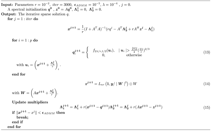
Algorithm 1. L_1/2QR PR: ADMM method for solving (4).

$\underset{q\in {ℝ}^n}{\min }\frac{1}{2}{\Vert q-u\Vert }_2^2+\mu {\Vert q\Vert }_{1/2}^{1/2}$ (16)

where $\mu >0$ . According to [19], the first-order stationary point definition of (16) is given as follow.

Definition 1. Let $\hat{q}$ be a vector in ${ℝ}^p$ and $Q=\text{Diag}\left(\hat{q}\right)$ where $\text{Diag}\left(\hat{q}\right)$ denotes a $p\times p$ diagonal matrix whose diagonal is formed by the vector $\hat{q}$ . The vector $\hat{q}$ is a first-order stationary point of (16) if

$Q\left(\hat{q}-u\right)+\frac{\mu }{2}{\left|\hat{q}\right|}^{1/2}=0.$

Similar to [20], we introduce the Karush-Kuhn-Tucker (KKT) conditions of the Lagrangian ${\mathcal{L}}_r\left(x\mathrm{,}q\mathrm{,}z\mathrm{<mo>\; ;\; </mo>}{\Lambda }_1\mathrm{,}{\Lambda }_2\right)$ in (2) as follows

$\{\begin{array}{l}{\partial }_x{\mathcal{L}}_r\left(\tilde{x}\mathrm{,}\tilde{q}\mathrm{,}\tilde{z}\mathrm{,}{\tilde{\Lambda }}_1\mathrm{,}{\tilde{\Lambda }}_2\right)=\mathrm{0,}\\ r\tilde{Q}\left(\tilde{q}-\tilde{x}+\frac{{\tilde{\Lambda }}_1}{r}\right)+\frac{\lambda }{2}{\left|\tilde{q}\right|}^{1/2}=\mathrm{0,}\\ {\partial }_z{\mathcal{L}}_r\left(\tilde{x}\mathrm{,}\tilde{q}\mathrm{,}\tilde{z}\mathrm{,}{\tilde{\Lambda }}_1\mathrm{,}{\tilde{\Lambda }}_2\right)=\mathrm{0,}\\ {\partial }_{{\Lambda }_1}{\mathcal{L}}_r\left(\tilde{x}\mathrm{,}\tilde{q}\mathrm{,}\tilde{z}\mathrm{,}{\tilde{\Lambda }}_1\mathrm{,}{\tilde{\Lambda }}_2\right)=\mathrm{0,}\\ {\partial }_{{\Lambda }_2}{\mathcal{L}}_r\left(\tilde{x}\mathrm{,}\tilde{q}\mathrm{,}\tilde{z}\mathrm{,}{\tilde{\Lambda }}_1\mathrm{,}{\tilde{\Lambda }}_2\right)=0\end{array}$ (17)

where $\left(\tilde{x}\mathrm{,}\tilde{q}\mathrm{,}\tilde{z}\mathrm{,}{\tilde{\Lambda }}_1\mathrm{,}{\tilde{\Lambda }}_2\right)$ is a saddle point, $\partial$ represents the partial derivative, $\tilde{q}=\text{Diag}\left(\tilde{q}\right)$ , $\tilde{q}$ is the first-order stationary point of q-subproblem (10).

Since the Lagrangian ${\mathcal{L}}_r\left(x\mathrm{,}q\mathrm{,}z\mathrm{<mo>\; ;\; </mo>}{\Lambda }_1\mathrm{,}{\Lambda }_2\right)$ is nonconvex w.r.t. $x\mathrm{,}q\mathrm{,}z$ . After analyzing the first-order optimality conditions for the variable z and the subproblem (12), the above KKT conditions corresponding to these three variables can be described as

$A^H{\tilde{\Lambda }}_2+{\tilde{\Lambda }}_1=\mathrm{0,}$

$\frac{\tilde{\Lambda }}{2}{\left|\tilde{q}\right|}^2-\tilde{Q}{\tilde{\Lambda }}_1=\mathrm{0,}$

$\left(\frac{2}{nr}sign\left({\left|{\tilde{z}}_m\right|}^2\right)-y_m\right){\tilde{z}}_m-{\left(\frac{{\tilde{\Lambda }}_2}{r}+A\tilde{x}\right)}_m\ni \mathrm{0,}m=\mathrm{1,2,3},\cdots \mathrm{,}n\mathrm{,}$

$\tilde{z}=A\tilde{x}\mathrm{,}$

$\tilde{x}=\tilde{q}\mathrm{,}$

where

$sign\left(\bar{x}\right)=\{\begin{array}{ll}\mathrm{1,}\hfill & \bar{x}\mathrm{<mo>\; >\; </mo>\; 0,}\hfill \\ -\mathrm{1,}\hfill & \bar{x}<\mathrm{0,}\hfill \\ \mathrm{0,}\hfill & \bar{x}<0.\hfill \end{array}$

Similar to Theorem 2.4 in [18], we show that our proposed algorithm converges to a saddle point satisfying KKT conditions.

Theorem 3. Assume that the successive differences of the two multipliers $\left\{{\Lambda }_1^j-{\Lambda }_1^{j-1}\mathrm{,}{\Lambda }_2^j-{\Lambda }_2^{j-1}\right\}$ converge to zero and $\left\{x^j\right\}$ is bounded. Then there exists a subsequence of iterative sequence of Algorithm 1 converging to an accumulation point that satisfies the KKT conditions of the saddle point problem (5).

3. Numerical Experiments

All simulations were performed on a 64-bit laptop computer running Windows 11 system with an AMD A8-6410 APU and 4 GB of RAM. To demonstrate the efficiency of our proposed method, we calculate the relative error between $x_{orig}$ and $\hat{x}$ as

$\text{Relative}\text{error}\mathrm{<mo>\; :\; </mo>}=\underset{c=\pm 1}{\min }\frac{{\Vert x_{orig}-\hat{x}\Vert }_2}{{\Vert x_{orig}\Vert }_2}\mathrm{,}$

where $x_{orig}$ is the true signal and $\hat{x}$ is the solution obtained by a solver. In all experiments, we carry out 100 Monte Carlo runs.

3.1. Experimental Parameters and Initialization

We take $p=128$ in all experiments, generating the true signal as Gaussian random sparse vector. The measurements matrix A generates from $a_i\stackrel{i\mathrm{.}i\mathrm{.}d\mathrm{.}}{\sim }\mathcal{N}\left(\mathrm{0,}I\right)$ . Regularization parameter $\lambda$ is given by a fixed 10⁻⁴. The penalty parameter r is chosen as 10⁻².

For nonconvex problems, ADMM can converge to different (and in particular, nonoptimal) points, depending on the initial values and the penalty parameter [21]. We take Wirtinger flow [22] with initial point $q^0$ , which obeys $\text{dist}\left(q^0\mathrm{,}x\right)\le \frac{1}{8}\Vert x\Vert$ , where $\text{dist}\left(q\mathrm{,}x\right)={\min }_{c=\pm 1}{\Vert q-cx\Vert }_2$ . Hence the algorithm proposed converges from the neighborhood of the global minimizer.

Like many phase retrieval methods, we use spectral initial values to achieve better recovery. To evaluate the efficiency of our method, we compare the successful recovery rate with 5 kinds of algorithm listed in Table 1.

Table 1. Comparison of reconstruction methods.

3.2. Success Rate Comparisons

We compare the recovery success rates of L_1/2QR PR at different values of $\tau$ in the noise-free case and noisy case including dense bounded noise and Laplace noise.

1) When not disturbed by noise, let $\tau =0.1,0.2,0.4,0.5,0.6,0.8,0.9$ . We report the success rates on Table 2 where the recovery is considered successful if the relative error is less than 0.0001.

2) When in dense bounded noise, let $\tau =0.1,0.2,0.4,0.5,0.6,0.8,0.9$ . The entries of the dense bounded noise are generated independently from $\mathcal{U}\left(0,{\eta }_{\max }\right)$ , where ${\eta }_{\max }/{\Vert x\Vert }_2=0.01$ . We say that the recovery is successful if the relative error is less than 0.001. Since the recovery success rate is 0 as $\tau =0.1$ , we here report the other cases on Table 3.

3) When in Laplace noise, let $\tau =0.4,0.5,0.6,0.8,0.9$ and $n/p=4,5,6$ . The entries of Laplace noise are generated from Laplace $\left(0,{\mu }_{\max }/\sqrt{2}\right)$ , where $\frac{{\mu }_{\max }}{{\Vert y\Vert }_2/\sqrt{n}}=0.001$ . We say that the recovery is successful if the relative error is less than 0.005 and report the success rate on Table 4.

From Tables 2-4, one can see that the recovery success rate of L_1/2QR PR with $\tau =0.5$ is usually better than when $\tau$ equals other values. For Laplace noise, L_1/2QR PR with $\tau =0.5$ and $\tau =0.8$ both perform well when $n/p=6$ .

Table 2. Success rate of L_1/2QR PR (Without noise).

Table 3. Success rate of L_1/2QR PR (Dense bounded noise).

Table 4. Success rate of L_1/2QR PR (Laplace noise).

Next, let’s continue to compare recovery success rate with the other five algorithms under different measurement fractions (n/p). We continue to use the same parameters and recovery success criteria as above. And let $\tau =0.5$ . Figure 1 shows how these algorithms behave without noise. Through repeated experiments, we find that median-MRWF has a better recovery success rate when measurement fractions (n/p) = 2, 3 and no noise interference in real field. The recovery success rate of L_1/2QR PR is slightly lower than that of median-RWF and median-MRWF, and higher than that of other algorithms. Figure 1 also shows how these algorithms behave when disturbed by noise. When receiving interference from dense bounded noise, the recovery success rate of L_1/2QR PR is higher than that of the other five algorithms in the real field. When receiving interference from laplace noise, the recovery success rate of L_1/2QR PR is higher than that of the other five algorithms in the real field.

In the following chapters, we make $\tau =0.5$ . And we fix the sparsity to s = 8 and use the competing algorithms listed in L_1/2QR PR the L₁ norm loss function, and L₀L₁PR adds L₀ regularization. The median-RWF and the median-MRAF of the L₂ norm loss function are highly robust to outliers through heuristic truncation rules. We compare the relative errors relative to the iteration count T under different measurement fractions (n/p), x is the true signal, x ^(t) is the tth iteration point.

Remark 3.1. We take n = 2p, 3p, 4p, 5p, 6p in real case. In detail, n = 2p and n = 4p are approximate theoretical sample complexity. When lad-admm returns to stability, we actually use n = 6p.

3.3. Exact Recovery for Noise-Free Data

In the noise-free case, Figure 2 shows in real case, when n = 2p, L_1/2QR PR and L_1/2LAD PR have good recovery performance. When n = 3p, 4p, 5p, 6p, L_1/2QR PR is slightly better than other 5 algorithms.

3.4. Stable Recovery with Dense Bounded Noise

Now, we consider the existence of dense bounded noise. The entries of the dense bounded noise are generated independently from $\mathcal{U}\left(0,{\eta }_{\max }\right)$ , where ${\eta }_{\max }/{\Vert x\Vert }_2=0.001,0.01$ . It can be seen from Figure 3, L_1/2QR PR shows great robustness to dense bounded noise in real case, while LAD-ADMM shows poor performance. L_1/2QR PR and L_1/2LAD PR have similar performance when n = 4p

(a)(b)(c)

Figure 1. Recovery success rate. (a) No noise; (b) Dense bounded noise; (c) Laplace noise.

(a) (b) (c) (d)

Figure 2. The relative error with respect to the iteration count for LAD-ADMM, median-RWF, median-MRAF, L₀L₁PR, L_1/2LAD PR, L_1/2QR PR with noise-free data in real case. (a) n = 2p; (b) n = 3p; (c) n = 5p; (d) n = 6p.

in real case. Median-RWF and median-MRAF have similar performance when n ≥ 4p in real case. Another reasonable observation, we find the relative reconstruction error has 10 times increase as η shrinks by a factor of 10 for all algorithms.

3.5. Stable Recovery with Laplace Noise

Finally, we consider the presence of Laplace noise, the entries of Laplace noise are generated from Laplace $\left(0,{\mu }_{\max }/\sqrt{2}\right)$ , where $\frac{{\mu }_{\max }}{{\Vert y\Vert }_2/\sqrt{n}}=0.001,0.01$ . As can be observed in Figure 4, surprisingly, L_1/2QR PR and L_1/2LAD PR are very robust to Laplace noise, especially in real case, no matter when n = 2p, 3p, 4p, 5p, 6p. However, other methods show poor performance, even when n = 6p, LAD-ADMM, L₀L₁PR, median-RWF, median-MRAF don’t have satisfactory recovery. Another logical observation, we find the relative reconstruction error has 10 times increase as ${\mu }_{\max }$ shrinks by a factor of 10 for all algorithms.

(a) (b) (c) (d) (e) (f)

Figure 3. The relative error with respect to the iteration count for LAD-ADMM, median-RWF, median-MRAF, L₀L₁PR, L_1/2LAD PR, and L_1/2QR PR with dense bounded noise in real case. ( $\eta =\frac{{\eta }_{\max }}{{\Vert x\Vert }_2}=0.001,0.01$ ). (a) n = 2p; η = 0.001; (b) n = 3p; η = 0.001; (c) n = 6p; η = 0.001; (d) n = 2p; η = 0.01; (e) n = 3p; η = 0.01; (f) n = 6p; η = 0.01.

(a) (b) (c) (d) (e) (f)

Figure 4. The relative error with respect to the iteration count for LAD-ADMM, median-RWF, median-MRAF, L₀L₁PR, L_1/2LAD PR, L_1/2QR PR with Laplace noise in real case. ( $\mu =\frac{{\mu }_{\max }}{{\Vert y\Vert }_2/\sqrt{n}}=0.001,0.01$ ). (a) n = 2p; η = 0.001; (b) n = 3p; η = 0.001; (c) n = 6p; η = 0.001; (d) n = 2p; η = 0.01; (e) n = 3p; η = 0.01; (f) n = 6p; η = 0.01.

The simulation results show that the L_1/2QR PR algorithm with quantile loss function and L_1/2 regularization has two significant advantages over other methods. One is the ability to recover the signal with fewer measured values, and the other is the robustness to asymmetrically distributed noise (such as dense bounded noise and Laplacian noise).

4. Conclusion

We proposed the L_1/2 QR PR method and designed an efficient algorithm based on the framework of ADMM. A series of numerical experiments show that the proposed method can recover sparse signals with fewer measurements and is robust to asymmetrically distributed noises such as dense bounded noises and Laplace noises. An interesting future research direction is to consider the complex situations, such as Fourier basic measurements, which is an application of coded diffraction patterns [26].

Acknowledgements

The authors would like to thank the editor and anonymous reviewers for their insight and helpful comments and suggestions which greatly improve the quality of the paper. The research was supported by the National Natural Science Foundation of China (NSFC) (11801130), the Natural Science Foundation of Hebei Province (A2019202135), the National Social Science Fund of China (17BSH140), “The Fundamental Research Funds for the Central Universities” in UIBE (16YB05) and “The Fundamental Research Funds for the Central Universities” (2022QNYL29).

NOTES

*Si Shen and Jiayao Xiang are joint first authors.

^#Corresponding author.

Conflicts of Interest

The authors declare no conflicts of interest regarding the publication of this paper.

References

[1]	Zhang, H., Chi, Y. and Liang, Y. (2018) Median-Truncated Nonconvex Approach for Phase Retrieval with Outliers. IEEE Transactions on Information Theory, 64, 7287-7310. https://doi.org/10.1109/TIT.2018.2847695
[2]	Cai, T.T., Li, X. and Ma, Z. (2016) Optimal Rates of Convergence for Noisy Sparse Phase Retrieval via Thresholded Wirtinger Flow. The Annals of Statistics, 44, 2221-2251. https://doi.org/10.1214/16-AOS1443
[3]	Ohlsson, H. and Eldar, Y.C. (2014) On Conditions for Uniqueness in Sparse Phase Retrieval. 2014 IEEE International Conference on Acoustics, Speech and Signal Processing, Florence, 4-9 May 2014, 1841-1845. https://doi.org/10.1109/ICASSP.2014.6853917
[4]	Hauptman, H.A. (1991) The Phase Problem of X-Ray Crystallography. Reports on Progress in Physics, 54, 1427-1454. https://doi.org/10.1088/0034-4885/54/11/002
[5]	Walther, A. (1963) The Question of Phase Retrieval in Optics. Optica Acta, 10, 41-49. https://doi.org/10.1080/713817747
[6]	Fan, J., Kong, L., Wang, L. and Xiu, N (2018) Variable Selection in Sparse Regression with Quadratic Measurements. Statistica Sinica, 28, 1157-1178. https://doi.org/10.5705/ss.202015.0335
[7]	Chang, H., Enfedaque, P. and Marchesini, S. (2019) Blind Ptychographic Phase Retrieval via Convergent Alternating Direction Method of Multipliers. SIAM Journal on Imaging Sciences, 12, 153-185. https://doi.org/10.1137/18M1188446
[8]	Candes, E.J., Strohmer, T. and Voroninski, V. (2013) PhaseLift: Exact and Stable Signal Recovery from Magnitude Measurements via Convex Programming. Communications on Pure and Applied Mathematics, 66, 1241-1274. https://doi.org/10.1002/cpa.21432
[9]	Xu, Z.B., Guo, H.L., Wang, Y. and Zhang, H. (2012) Representative of L1/2 Regularization Among Lq (0 ≤ q ≤ 1) Regularizations: An Experimental Study Based on Phase Diagram, Automatica Sinica, 38, 1225-1228. (In Chinese) https://doi.org/10.3724/SP.J.1004.2012.01225
[10]	Zhang, H., Zhou, Y., Liang, Y. and Chi, Y. (2017) A Nonconvex Approach for Phase Retrieval: Reshaped Wirtinger Flow and Incremental Algorithms. Journal of Machine Learning Research, 18, 1-35.
[11]	Yan, A. and Song, F. (2019) Adaptive Elastic Net-Penalized Quantile Regression for Variable Selection. Communications in Statistics-Theory and Methods, 48, 5106-5120. https://doi.org/10.1080/03610926.2018.1508711
[12]	Song, Y., Jian, L. and Lin, L. (2016) Robust Exponential Squared Loss-Based Variable Selection for High-Dimensional Single-Index Varying-Coefficient Model. Journal of Computational and Applied Mathematics, 308, 330-345. https://doi.org/10.1016/j.cam.2016.05.030
[13]	Kurnaz, F. S., Hoffmann, I. and Filzmoser, P. (2018) Robust and Sparse Estimation Methods for High Dimensional Linear and Logistic Regression. Chemometrics and Intelligent Laboratory Systems, 172, 211-222. https://doi.org/10.1016/j.chemolab.2017.11.017
[14]	Ciuperca, G. (2017) Adaptive Fused LASSO in Grouped Quantile Regression. Journal of Statistical Theory and Practice, 11, 107-125. https://doi.org/10.1080/15598608.2016.1258601
[15]	Gu, Y., Fan, J., Kong, L., Ma, S. and Zou, H. (2018) ADMM for High-Dimensional Sparse Penalized Quantile Regression. Technometrics, 60, 319-331. https://doi.org/10.1080/00401706.2017.1345703
[16]	Xu, Z., Chang, X., Xu, F. and Zhang, H. (2012) L1/2 Regularization: A Thresholding Representation Theory and a Fast Solver. IEEE Transactions on Neural Networks and Learning Systems, 23, 1013-1027. https://doi.org/10.1109/TNNLS.2012.2197412
[17]	Zeng, J.S., Fang, J. and Xu, Z.B. (2012) Sparse SAR Imaging Based on L1/2 Regularization. Science China Information Sciences, 55, 1755-1775. https://doi.org/10.1007/s11432-012-4632-5
[18]	Kong, L.J., Yan, A.L., Li, Y. and Fan, J. (2022) L1/2-Regularized Least Absolute Deviation Method for Sparse Phase Retrieval. Pacific Journal of Optimization, 18, 213-232.
[19]	Dhifallah, O. and Lu, Y.M. (2017) Fundamental Limits of PhaseMax for Phase Retrieval: A Replica Analysis. 2017 IEEE 7th International Workshop on Computational Advances in Multi-Sensor Adaptive Processing (CAMSAP), Curacao, 10-13 December 2017, 1-5. https://doi.org/10.1109/CAMSAP.2017.8313210
[20]	Chang, H., Lou, Y., Duan, Y. and Marchesini, S. (2018) Total Variation-Based Phase Retrieval for Poisson Noise Removal. SIAM Journal on Imaging Sciences, 11, 24-55. https://doi.org/10.1137/16M1103270
[21]	Boyd, S., Parikh, N., Chu, E., Peleato, B. and Eckstein, J. (2010) Distributed Optimization and Statistical Learning via the Alternating Direction Method of Multipliers. Foundations and Trends in Machine Learning, 3, 1-122. https://doi.org/10.1561/2200000016
[22]	Candes, E. J., Li, X. and Soltanolkotabi, M. (2015) Phase Retrieval via Wirtinger Flow: Theory and Algorithms. IEEE Transactions on Information Theory, 61, 1985-2007. https://doi.org/10.1109/TIT.2015.2399924
[23]	Duan, Y., Wu, C., Pang, Z. F. and Chang, H. (2016) L0-Regularized Variational Methods for Sparse Phase Retrieval. ArXiv: 1612.02538.
[24]	Jiang, X., So, H.C. and Liu, X. (2020) Robust Phase Retrieval with Outliers. ICASSP 2020-2020 IEEE International Conference on Acoustics, Speech and Signal Processing (ICASSP), Barcelona, 4-8 May 2020, 5320-5324. https://doi.org/10.1109/ICASSP40776.2020.9053060
[25]	Zhang, Q., Liu, D., Hu, F., Li, A. and Cheng, H. (2021) Median Momentum Reweighted Amplitude Flow for Phase Retrieval with Arbitrary Corruption. Journal of Modern Optics, 68, 374-381. https://doi.org/10.1080/09500340.2021.1897171
[26]	Candes, E.J., Li, X. and Soltanolkotabi, M. (2015) Phase Retrieval from Coded Diffraction Patterns. Applied and Computational Harmonic Analysis, 39, 277-299. https://doi.org/10.1016/j.acha.2014.09.004