A Geometric Formulation and a Series Approach for Estimating π with Remarks on a Sumerian Tablet

Serdar Beji

Faculty of Naval Architecture and Ocean Engineering, Istanbul Technical University, Istanbul, Turkey.

DOI: 10.4236/apm.2022.1211045                

Abstract

A recursive method based on successive computations of perimeters of inscribed regular polygons for estimating π is formulated by employing the Pythagorean theorem alone without resorting to any trigonometric calculations. The approach is classical but the formulation of coupled recursion relations is new. Further, use of infinite series for computing π is explored by an improved version of Leibniz’s series expansion. Finally, some remarks with reference to π are made on a relatively recently rediscovered Sumerian tablet depicting geometric figures.

Keywords

π from Recursive Formulas for Polygonal Perimeters, Arayabatha’s Method of Estimating π, Improved Leibniz Series for Computing π, Sumerian Tablet of Geometric Figures

1. Introduction

Archimedes (287-212 B.C.) of Syracuse, the first of three greatest mathematicians ever according to Gauss (1777-1855), made indelible contributions to not only mathematics but every branch of mechanics [1] . Besides giving a method for

computing π, and showing that for a regular polygon of 96 sides $\frac{223}{71}<\pi <\frac{22}{7}$ ,

Archimedes formulated an ingenious way of calculating the segment area of a parabola ( [2] , p. 6).

Quite a number of mathematicians tackled with the problem of accurate computation of π but none devoted a lifetime like Ludolph Van Ceulen (1540-1610), whose forename was used to indicate π as Ludolphine number for a long period in Germany [1] . Following Archimedes, by way of computing the circumference of a regular polygon of 15 × 2³¹ sides, in 1596 Van Ceulen gave π correct to 20 decimal places. After Van Ceulen’s death first a 33 decimal-place-correct π in 1615 and then his ultimate work of 35 decimal-place-approximation was published in 1621 from his works. Lower and upper bounds of π with 35 decimals were engraved on Van Ceulen’s tombstone as a tribute to his lifetime devotion to this number.

The present work diverges from the Archimedes’ frequently used path in two ways. First, instead of using both inscribed and circumscribed regular polygons for establishing lower and upper bounds for π, only inscribed polygons with successively doubling sides are used to improve the estimate of π at each step; a method originally used by the Hindus ( [3] , p. 23). Second, starting from a triangle or a square, two coupled recursive formulas written directly from the Pythagorean theorem are used for computing the perimeters of inscribed polygons of successively doubling sides without resorting to any trigonometric calculation. Reformulation of an ancient problem by relatively modern techniques can be done in various ways but a somewhat meaningful contribution can only be achieved by producing a method that uses only the means available in those times. It is trivial to write the perimeter p of an $3\cdot 2^n$ -sided polygon $p=3\cdot 2^{n+1}R\sin \left(180˚/3\cdot 2^n\right)$ where $n=1,2,\cdots$ and $n=1$ corresponds to a hexagon giving the familiar answer $\pi \simeq 3$ for an estimate. But this formula requires calculation of sine function (or in the past tables of sine function as used by Van Ceulen) for each n value. This is the main reason of intentional avoidance of trigonometric functions in the present approach. Accordingly, the resulting formulation is simple enough for an expository treatment of this ancient problem at elementary level with no other knowledge than the Pythagorean theorem and related square root operations.

In Section 3, the historically first infinite series approximation to π is appreciably improved and computed results up to 50 terms and 15 decimal places accuracy are presented.

The final part of the work reveals some rather interesting features concerning the overall geometric arrangement of a rediscovered ancient Sumerian tablet by establishing definite dimensionless ratios.

2. Approximate Determination of Circle Perimeter from Perimeters of Successively Generated Polygons

The approach used here is an ancient method of estimating π by computing the perimeters of successively generated regular polygons. By employing this method and starting from the natural choice of a hexagon for which the side length is equal to the radius of circumscribing circle, Arayabatha ( [3] , p. 23) used the formula $s^2\left(2n\right)=2-\sqrt{4-s^2\left(n\right)}$ for computing the perimeter of a polygon with 384 sides and gave the estimate for π as $\sqrt{98694}/100=3.14156\cdots$ ¹. The

Table 1. Twenty six steps of computations starting from a triangle by use of (1) and (2) for estimating π correct to 15 decimal places. Incorrect digits are colored red.

present work follows a simple didactic approach and derives two coupled recursion formulas as a new contribution for computing the side lengths of regular polygons of successively doubled sides.

2.1. Polygons Generated from a Triangle

Figure 1 shows a succession of inscribed polygons generated by drawing smaller triangles to every side of a main triangle centered in a circle. Thus, starting with an inscribed triangle and then creating a hexagon (6-gon), a dodecagon (12-gon), icositetragon (24-gon), etc., polygons of $3\cdot 2^{n-1}$ sides are generated for $n=1,2,3,\cdots$ .

Figure 1. Successive generation of regular polygons starting from an equilateral triangle (black) for a circumscribing circle of radius r₀.

The side-length s₁ of the main equilateral triangle in Figure 1 can be easily obtained in terms of the given circumradius r₀ by employing the Pythagorean theorem together with the relation $r_1=r_0/2$ so that for the initial stage of calculations

$s_1=\sqrt{3}{r}_0,r_1=r_0/2.$ (1)

Keeping these starting values at our disposal we proceed to express s₂ and r₂ of the hexagon as $s_2^2={\left(s_1/2\right)}^2+{\left(r_0-r_1\right)}^2$ and $r_2^2=r_0^2-{\left(s_2/2\right)}^2$ . Note that s₂ can be computed from s₁ and r₁, and then used for computing r₂. Generalization of these expressions to two coupled recursive formulas is straightforward

$s_{n+1}^2={\left(s_n/2\right)}^2+{\left(r_0-r_n\right)}^2,r_{n+1}^2=r_0^2-{\left(s_{n+1}/2\right)}^2,$ (2)

where $n=1,2,3,\cdots$ . Beginning with the known s₁ and r₁ values, the successive use of recursive couple in (2) enables one to compute the side-length s_n of a polygon for any desired number of sides $3\cdot 2^{n-1}$ as far as the machine capabilities allow. The corresponding perimeter of the polygon is $p_n=\left(3\cdot 2^{n-1}\right)\cdot s_n$ hence the estimate for $\pi \simeq p_n/2r_0$ .

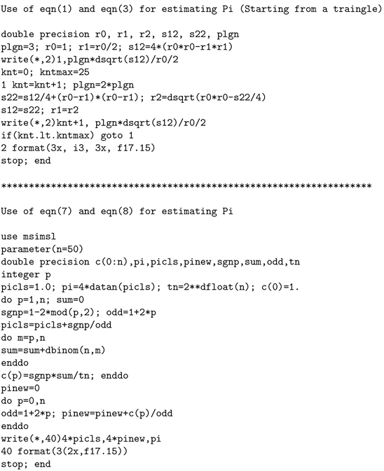
A short FORTRAN program making use of Equations (1) and (2) for successive computations is provided in the Appendix. Table 1 gives the results of twenty six steps, starting from perimeter p₁ of the main triangle to perimeter p₂₆ of the $3\cdot 2^{25}$ -sided polygon. The reason for restricting the computations to this range is that the double precision operations are performed for 16 digits and at the 26th step π is estimated correct to 15 decimal places; adding one digit for the whole part totals to 16 digits. Further computations are futile as no improvement is possible with the available computational capabilities. Estimates of π from these regular polygons are given in the last column of Table 1. The numbers in red are incorrect digits; note that as a number starts repeating in succeeding iterations it can be identified as correct without resorting to any other source. An interesting point is observed at the second iteration where a hexagon is generated. In this particular case the side length is equal to r₀ and therefore the perimeter becomes 6r₀, resulting in the estimate $\pi \simeq 6r_0/2r_0=3$ , exactly as pointed out previously.

2.2. Polygons Generated from a Square

Instead of a triangle we are going to begin with a square now. Figure 2 shows polygons generated by drawing triangles to every side of a square (regular quadrilateral) centered in a circle. Hence, starting with an inscribed square then drawing a octagon (8-gon), a hexadecagon (16-gon), etc., polygons of $4\cdot 2^{n-1}$ sides are generated for $n=1,2,3,\cdots$ .

The side-length s₁ of the square in Figure 2 and the distance r₁ are obviously

$s_1=\sqrt{2}{r}_0,r_1=\sqrt{2}{r}_0/2$ (3)

Figure 2. Successive generation of regular polygons starting from a square for a circumscribing circle of radius r₀.

where r₀ is the circumradius. We now make use of starting values s₁ and r₁ given in (3) and then use the recursion relations of (2) for successive computations. The computer program used is identical with the first one except for the starting values s₁ and r₁ hence is not given again. Table 2 gives the results of twenty five steps, starting from p₁ of the square to p₂₅ of the $4\cdot 2^{24}$ -sided polygon. Estimates of π from these regular polygons are given in the last column. Note that starting from a square instead of triangle saved only a single step in reaching the same degree of accuracy. Going on further and starting from a pentagon would likewise not make an appreciable saving either while requiring the use of trigonometric relations to initiate the computations, s₁ and r₁.

Table 2. Twenty five steps of computations starting from a square by use of (2) and (3) for estimating πcorrect to 15 decimal places. Incorrect digits are colored red.

3. Series Expansions for Estimating π

We begin by recalling the well-known integral

${\displaystyle {\int }_0^1}\frac{\text{d}x}{1+x^2}={\left[\arctan \left(x\right)\right]}_0^1=\arctan \left(1\right)-\arctan \left(0\right)=\frac{\pi }{4}$ (4)

To evaluate the integral numerically two different series expansions are employed. The first one is the standard expansion obtained from either simple division or Maclaurin series,

$\frac{1}{1+x^2}=1+{\displaystyle \underset{p=1}{\overset{n}{\sum }}}{\left(-1\right)}^p{x}^{2p}\text{for}x\le 1$ (5)

which in a sense is a deficient representation of $1/1+x^2$ due to the paradox encountered for $x=1$ . The second expression is a rectified and convergence improved expansion obtained from a satisfactory resolution to this paradox [4] [5] ,

$\frac{1}{1+x^2}=1+\frac{1}{2^n}{\displaystyle \underset{p=1}{\overset{n}{\sum }}}\left[{\displaystyle \underset{m=p}{\overset{n}{\sum }}}\left(\begin{array}{c}n\\ m\end{array}\right)\right]{\left(-1\right)}^p{x}^{2p}\text{for}x\le 1$ (6)

where n is an arbitrary truncation order. Integrating (5) and (6) from 0 to 1 gives respectively

$\frac{\pi }{4}=1+{\displaystyle \underset{p=1}{\overset{n}{\sum }}}\frac{{\left(-1\right)}^p}{2p+1}$ (7)

$\frac{\pi }{4}=1+\frac{1}{2^n}{\displaystyle \underset{p=1}{\overset{n}{\sum }}}\left[{\displaystyle \underset{m=p}{\overset{n}{\sum }}}\left(\begin{array}{c}n\\ m\end{array}\right)\right]\frac{{\left(-1\right)}^p}{2p+1}$ (8)

For $n=5$ we get the following estimates from the standard and improved series

$\pi \simeq 4\left(1-\frac{1}{3}+\frac{1}{5}-\frac{1}{7}+\frac{1}{9}-\frac{1}{11}\right)=2.976046$ (9)

$\pi \simeq 4\left(1-\frac{31}{32}\frac{1}{3}+\frac{26}{32}\frac{1}{5}-\frac{16}{32}\frac{1}{7}+\frac{6}{32}\frac{1}{9}-\frac{1}{32}\frac{1}{11}\right)=3.144588$ (10)

which have respectively −5.3% and 0.1% relative errors, revealing that the improved series performs remarkably well compared to the standard approach. We remark here that the classic series representation of π, originally given by Leibniz (1646-1716) was the first infinite series derived for estimating π ( [2] , p. 10) and ( [3] , p. 149).

Table 3 lists π estimates computed for $n=5,10,\cdots ,50$ terms according to the classic and improved formulations. The standard series converges very slowly; indeed its convergence is notoriously slow that even 300 terms are insufficient to obtain two decimal places of accuracy. On the other hand, the same series in improved form performs quite well and actually reaches 15 decimal place accuracy for $n=49$ terms. It must however be admitted that the present convergence-improved series is inferior to the estimate of Isaac Newton (1643-1727), which attains the same accuracy by the use of $n=22$ terms of a series representing

Table 3. Estimates of π for $n=5,10,\cdots ,50$ terms as computed from the standard (7) and improved (8) formulations. Incorrect numbers are colored red.

area of a circular arc ( [3] , p. 160). Nevertheless, the present formulation, (8), deserves credit for enormously improving a practically useless series expansion of (7).

The recursion formulas and the series expansion approach presented here are at the elementary level with modest achievements. They cannot compete at all with very successful schemes such as the Gauss-Legendre iterative algorithm, the Ramanujan or Chudnovsky formulas, which are far beyond the classical series, producing computations of π correct to trillions of digits. Also, there are the so-called spigot algorithms which produce single digits of π that are not reused once calculated. These approaches are quite different from infinite series or iterative algorithms in which all intermediate digits are kept to produce the final result. Our aim here is simply to present new formulations to the classic approaches.

4. A Sumerian Tablet

Sumerians established the oldest civilization known in the southern Mesopotamia (today’s south-central Iraq) between the sixth and fifth millennium BC and continued to reign till around 1900 BC. Proto-writing originated from the cities of Sumer between 3500-3000 BC and the world’s oldest literary achievement the “Epic of Gilgamesh” was written there as an epic poem in cuneiform on 12 clay tablets in about 2200 BC thus pre-dating Homer’s Iliad by nearly a millennium and a half. Sumerians were quite advanced in mathematics for their time, knowing and using the so-called “Pythagorean theorem” thousands of years before Pythagoras was born and formulating the roots of second-order polynomials.

Sumerians used a sexagesimal, base 60, number system in line with the one used for maps today. For instance 08:25:19 corresponds to $08\times {60}^2+25\times 60+19=30319$ in our base 10 system, though some ambiguity may arise as explained in [6] . Considerable research effort has gone into deciphering the tablets remained from Sumerians. Quite recently, Mansfield [6] has done an extensive study of a mathematically remarkable Sumerian tablet named Plimpton 322 and arrived at rather new conclusions concerning the purpose of such tablets. To support his conjectures Mansfield examined another tablet called Si.427, shown in Figure 3. This particular tablet was in a sense rediscovered by Mansfield though it had been acquired by Istanbul Archaeology Museum about 100 years earlier. From the study of Plimpton 322 and Si.427 Mansfield concludes that Sumerians basically aimed at improved cadastral surveying of land and used diagonal triples (Pythagorean triples) to create accurate perpendicular lines in apportioning a field. Interested reader is directed to [6] [7] for a thorough exposition of these tablets with convincing arguments regarding their purposes of use.

We consider Si.427 from a different viewpoint and examine its geometric properties rather than its contents by establishing definite ratios or non-dimensional numbers. First, the lines on Si.427 are traced with light gray color to clarify their appearance and then a chord c_b (gray) and two sagittas s_t,s_b (red) added as shown in Figure 4. All these drawings could be done approximately; likewise, the lengths indicated, a, b, c, $\cdots$ , could not be measured precisely. More importantly, the tablet itself is of baked clay with imperfections of form due to production defects, possible deformations by thermal stresses in baking, and finally abrasive effects of thousands of years. Being broken into two pieces adds an extra

Figure 3. Photograph of Si.427. Courtesy of Istanbul Archaeology Museum (İstanbul Arkeoloji Müzesi).

Figure 4. Original lines on Si.427 traced (light gray) and a chord (gray) and two sagittas (red) added.

element of inaccuracy to the measurements. For all these reasons the statements concerning lengths hence ratios must necessarily be taken as approximate and our inclination to round off the numbers in some places should be borne with tolerance.

First, measurements of diameter in four different compass directions, North-South (N-S), Northeast-Southwest (NE-SW), East-West (E-W), and Northwest-Southeast (NW-SE), were made from the photograph of Si.427 at an arbitrary scale. Then, the average of these measurements was calculated and converted to the true size by the use of measure given in the photograph. The average diameter thus obtained for Si.427 tablet in actual size is $D=102.82\text{mm}$ .

A rather simple survey of definite ratios is considered here. To this purpose the sagitta s_t at the top drawn to the chord c_t and the sagitta s_b drawn to the chord c_b established at the bottom are of interest to us. Measuring s_t and s_b and then calculating c_t and c_b by the use of mean diameter give $s_t=14.72\text{mm}$ , $c_t=72.02\text{mm}$ and $s_b=29.12\text{mm}$ , $c_b=92.62\text{mm}$ . Hence one can establish the following dimensionless ratios:

$\frac{s_t}{D}=0.142996,\frac{s_b}{2D}=0.141537$ (11)

Viewing these decimals, the first ratio compels the mind to relate it to the quotient $1/7\simeq 0.142857$ , which could lead to $\pi -3\simeq 1/7$ hence $\pi \simeq 22/7$ , the well-known approximation to π. On the other hand, the second ratio can likewise be related to the more accurate difference $\pi -3=0.141593$ . All these implications can of course be purely coincidental but the near repetition of the same decimals for both $s_t/D$ and $s_b/2D$ makes it less likely. From another aspect, assuming random selections for the location of top chord and the baseline of the main figures would not be convincing when a relevance can be established between these two choices. Nevertheless, it must be admitted that no conclusive decision can be made.

We now move on to establish some other ratios for the mere purpose of revealing some hints to the sexagesimal number system used by Sumerians. First, the ratios $D/c_t$ and $D/c_b$ are considered by introducing a very fine adjustment to $c_b$ so that in place of the measured value $c_b=92.62\text{mm}$ we take $c_b=92.522\text{mm}$ for getting a simpler fraction in the end.

$\frac{D}{c_t}=\frac{102.8}{72}=\frac{257}{180}=\frac{04:17}{03:00},\frac{D}{c_b}=\frac{102.8}{92.52}=\frac{200}{180}=\frac{03:20}{03:00}$ (12)

where the last ratios are expressed in sexagesimal system. Moreover, in view of possible measurement inaccuracies $D/c_t=257/180$ could well be $260/180=\mathrm{04\; <mo>\; :\; </mo>\; 20}/\mathrm{03\; <mo>\; :\; </mo>\; 00}$ and this ratio is now well associated with $D/c_b=03:20/03:00$ when viewed in sexagesimal system. However, such possibilities are not vitally important as the appearance of $180=3\times 60=03:00$ in the denominators should be a good enough implication of the sexagesimal system.

Next consider the big triangle on the right side of Si.427 with measured approximate lengths of $a=17.942\text{mm}$ , $b=42.942\text{mm}$ , and $c=45.882\text{mm}$ . This is a triangle of $\left(\mathrm{5,12,13}\right)$ triples as Mansfield [7] indicated2. To comply with $\left(\mathrm{5,12,13}\right)$ triples exactly, the side lengths of the triangle are redefined as $a=18.02\text{mm}$ , $b=43.22\text{mm}$ , and $c=46.82\text{mm}$ . Since all the lengths are increased to some extent the diameter is likewise set to $D=104.02\text{mm}$ instead of $D=102.82\text{mm}$ .

$\frac{a}{D}=\frac{45}{260}=\frac{00:45}{04:20},\frac{b}{D}=\frac{108}{260}=\frac{01:48}{04:20},\frac{c}{D}=\frac{117}{260}=\frac{01:57}{04:20}$ (13)

Notice that the last ratio $c/D=117/260=0.45$ is half the ratio $c_b/D=180/200=0.90$ hence indicating that $c=c_b/2$ . Since all the ratios with some relevance to each other are obtained only by some minor variations of the measured values, we may attribute them to premeditated arrangements rather than arbitrary choices.

In closing, we are aware that the square on the left in Figure 4 does not exactly have the side length a; likewise, two small squares with sides q are not quite square and two small triangles are not exactly the same with sides a and q; but all these values are ascribed to them as being the most approximate ones within the uncertainties involved. More importantly, works of the true expert Mansfield [6] [7] focus on quite practical implications since Si.427 “concerns the sale of private land with unusually high precision measurements”; hence, our speculative treatment may only be viewed as something interesting to contemplate.

5. Concluding Remarks

An ancient method based on regular polygons of doubling sides is reformulated by introducing new recursive equations to estimate π by successive approximations. To the same purpose, the historically first series approximation to π is improved remarkably and computational results with various degrees of accuracy are presented. Finally, some remarks on a relatively recently rediscovered Sumerian tablet are made from purely geometric arrangement viewpoint.

Appendix

NOTES

¹This value is the same as the one computed at the eight iteration for $3\cdot 2^7=384$ sides polygon in Table 1.

²Mansfield also indicates the use of (8, 15, 17) triples on Si.427; however, we could not detect it for the smaller triangles; all appeared to comply with (5, 12, 13) triples.

Conflicts of Interest

The author declares no conflicts of interest regarding the publication of this paper.

References

[1]	O’Conner, J.J. and Robertson, E.F. (2022) McTutor History of Mathematics Archive. http://www-history.mcs.st-andrews.ac.uk
[2]	Burk, F.E. (2007) A Garden of Integrals. The Mathematical Association of America, Washington DC, Vol. 31. https://doi.org/10.7135/UPO9781614442097
[3]	Beckmann, P. (1971) A History of π (Pi). St. Martin’s Press, New York.
[4]	Beji, S. (2020) Resolution of Grandi’s Paradox and Investigations on Related Series. Applied Mathematics E-Notes, 20, 265-277.
[5]	Beji, S. (2020) Resolution of Grandi’s Paradox as Extended to Complex Valued Functions. Advances in Pure Mathematics, 10, 447-463. https://doi.org/10.4236/apm.2020.108027
[6]	Mansfield, D.F. (2020) Perpendicular Lines and Diagonal Triples in Old Babylonian Surveying. Journal of Cuneiform Studies, 72, 87-99. https://doi.org/10.1086/709309
[7]	Mansfield, D.F. (2021) Plimpton 322: A Study of Rectangles. Foundations of Science, 26, 977-1005. https://doi.org/10.1007/s10699-021-09806-0