Approximating Ordinary Differential Equations by Means of the Chess Game Moves

Maria Teresa Signes-Pont, Joan Boters-Pitarch, José Juan Cortés-Plana, Higinio Mora-Mora

Department of Computer Science and Technology, University of Alicante, Alicante, Spain.

DOI: 10.4236/jamp.2022.1010215                

Abstract

The chess game provides a very rich experience in neighborhood types. The chess pieces have vertical, horizontal, diagonal, up/down or combined movements on one or many squares of the chess. These movements can associate with neighborhoods. Our work aims to set a behavioral approximation between calculations carried out by means of traditional computation tools such as ordinary differential equations (ODEs) and the evolution of the value of the cells caused by the chess game moves. Our proposal is based on a grid. The cells’ value changes as time pass depending on both their neighborhood and an update rule. This framework succeeds in applying real data matching in the cases of the ODEs used in compartmental models of disease expansion, such as the well-known Susceptible-Infected Recovered (SIR) model and its derivatives, as well as in the case of population dynamics in competition for resources, depicted by the Lotke-Volterra model.

Keywords

Chess Game, Neighborhood, Update Rule, ODE, SIR Model, Lotke-Volterra Model

1. Introduction

Though forms of the board game, now known as chess, have existed since the sixth century, it took nearly a thousand years for the pieces used in the game to reach their modern form. While the rules governing these pieces may be relatively straightforward, the relationships between them are complex [1]. In this work, we are interested in the movement of the different pieces: pawn, knight, bishop, rook, queen and king.

Table 1 summarizes the rules of chess. As we see, the main moves are vertical (forward/backward), horizontal (forward/backward), diagonal (forward/backward),

Table 1. The rules of chess.

all of them with one or more than one square length, and finally Knight (L) moves in a combination of vertical/horizontal moves, with 1 and 2 or 2 and 1 squares length, respectively.

In terms of cellular automata [2], the von Neumann neighborhood (or 4-neighborhood) is classically defined on a two-dimensional square grid and is composed of a central cell and its four adjacent cells that are at a Manhattan distance of 1. It is named after John von Neumann, who used it to define both the von Neumann cellular automaton and the universal constructor within it. This recalls the rook basal move (R) of the chess game when the step length is equal to one square. The second most used neighborhood is the Moore neighborhood. It is named after Edward F. Moore, a pioneer of cellular automata theory. In cellular automata, the Moore neighborhood is defined on a two-dimensional square grid and is composed of a central cell and the eight cells that surround it (8-neighbours) that are at a Chebyshev distance of 1. It is similar to the notion of 8-connected pixels in computer graphics. The well-known Conway’s Game of Life, for example, uses the Moore neighborhood. This could be compared to the king move of the chess game (K). In this paper, we also define the Diagonal neighborhood, based on the bishop basal move (B) with a step length equal to one, and the L neighborhood, shaped on the knight moves. Figure 1 shows four neighborhoods (R, K, B and L) that can be implemented by the basal moves of the chess game.

Figure 1. Basal moves of the chess game implementing R, K, B and L neighborhoods.

The central cell is set to 1 and then, the 1 value extends to the neighbor cells that are initially set to 0.

In this paper, we are interested in exploring the capabilities of the movements of the chess pieces to define a new way to perform operations that provide a behavioral approximation to the calculations carried out by means of traditional computation tools such as ordinary differential equations (ODEs). Our proposal is based on a grid. The cells value changes as time pass depending on both a neighborhood and an update rule. This framework succeeds in applying real data matching in the cases of the ODEs used in compartmental models of disease expansion, such as the well-known Susceptible-Infected Recovered (SIR) model and its derivatives, as well as for population dynamics in competition for resources, such as the Lotke-Volterra model.

Following the Introduction, Section 2 presents the rules for operating in the grid. Section3 provides examples of running spread patterns with their graphical representation. Section 4 completes the model by adding the delays in the application of the rules. Section 5 is dedicated to reporting on the state of the art of the ODE and discusses recent advances in improvements. Three examples are presented related to SIR, SIS and Lotka-Volterra models. Section 6 summarizes and presents concluding remarks and future lines of investigation.

2. Building Update Rules

Each cell of the grid has an initial value which is 0 or 1. An update rule is needed when having to define the values of the cells at any time. In this work, the calculation step is defined as a generation, which is a generic time that recalls the evolution of living beings. The generation may be worth one minute, one hour, or one year, depending on the dynamics of the application considered. Criteria for the changes in values must also be provided. The changes in the cells can be triggered by the change of a cell, which “infects” its neighbor cells. These neighbor cells follow the same “infection” pattern and spread the changes throughout all grid later. Nevertheless, some changes may be spontaneous.

We can define 2⁴ = 16 different update rules. The formal definition is as follows:

Let “a” be a cell in the grid, and f(a) its value (f(a) = 0 or f(a) = 1),

Let V(a) be the set of the neighbors of a cell,

Let U_m be an update rule ( $m\in \left[0,15\right]$ ).

$\forall b,b\in V\left(a\right)/U_m\left(a,b\right)=f\left(a\right)\ast f(\; b\; )$

This operator means that f(a) updates the value of the cell b, f(b).

The initial value f(a) is given or spontaneously updated.

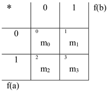
The 16 different update rules U_m come straightforward from the following consideration:

$U_m\left(a,b\right)=f\left(a\right)\ast f\left(b\right)=m_i$,with $i\in \left[1,3\right]$

The sequence m = m₃ m₂ m₁ m₀ defines the possible values for f(a) * f(b) when f(a) and f(b) take values in [0, 1].

As an example, U₇ corresponds to m₃ = 1, m₂ = 1, m₁ = 1, m₀ = 0, that is to say:

$m_3=1\ast 1=1$ ;

$m_2=1\ast 0=1$ ;

$m_1=0\ast 1=1$ ;

and $m_0=0\ast 0=0$.

3. Running a Spread Pattern

The running conditions of a spread pattern are:

● The square grid has a finite size, n × n.

● The spread S is characterized by (m, V), where $m\in \left[0,2^4\right]$ and $V\in \left[\text{R},\text{K},\text{B},\text{L}\right]$.

● The spread can go forward and/or backward.

● The initial values of the cells in the grid are known.

3.1. Graphical Representation of S (14, R)

We consider 10 × 10 and 100 × 100 grids. The spread defines two different classes of cells, namely Susceptible (value = 0) and Infected (value = 1). At generation = 0, the central cell a has a value f(a) = 1 (infected) and all other cells in the lattice are set to 0 (susceptible). The scheme of this spread is given by the rule U₁₄:

m₃ = 1, this means 1 × 1 = 1;

m₂ = 1, this means 1 × 0 = 1;

m₁ = 1, this means 0 × 1 = 1;

m₀ = 0, this means 0 × 0 = 0.

R neighborhood has been chosen. Figure 2 shows the spread pattern of S(14, R) at any time.

We can make some remarks:

The same behavior could have been observed with a forward/backward spread because U₁₄ avoids backward execution to have any effect on the spread. The spread follows a diamond shape evolution, see Figure 1. The number of changes N is carried out by the recursive Equation (1):

$N_g=N_{g-1}+4g$ (1)

g stands for the generation number and N₀= 1

As N_max = n × n (grid size), the number N_g converges to a horizontal asymptote equal to N_max. The grid size has no effect on the spread except for the delay in achieving N_max.

3.2. Graphical Representation of S(14, K)

We consider a 10 × 10 and 100 × 100 grids.

At generation = 0, the central cell a has a value f(a) = 1 and all other cells in the grid are set to 0.

We consider first a forward spread for K neighborhood.

The scheme of this spread is given by the rule U₁₄ (see section 3.1).

Figure 3 shows the spread pattern of S(14, K) at any time.

We can make some remarks:

The same behavior could have been observed with a forward/backward spread because U₁₄ avoids backward execution to have any effect on the spread. The

Figure 2. Spread pattern of S(14, R) at any time in grids 10 × 10 and 100 × 100.

Figure 3. Spread pattern of S(14, K) at any time in grids 10 × 10 and 100 × 100.

spread follows a square shape evolution, see Figure 1. The number of changes N_g is carried out by the recursive Equation (2):

$N_g=N_{g-1}+8g$ (2)

g is the generation number andN₀ = 1

As N_max = n × n (grid size), the number N_g converges to a horizontal asymptote.

The grid size has no effect on the spread, except for the delay to achieve N_max.

3.3. Graphical Representation of S(14, L)

The running conditions are the same as in 3.1 and 3.2.

Figure 4 shows the spread pattern of S (14, L) at any time.

The spread follows a regular square alternate shape evolution. The number of changes N is carried out by the recursive Equation (3):

$N_g=N_{g-1}+2^{2g+1}$ (3)

gis the generation number and N₀ = 1.

As N_max = n × n (grid size), the number N_g converges to a horizontal asymptote.

The representation of S(14, B) has been omitted because it is the same as for S(14, R). The comparison between the three neighborhoods shows the evolution in R neighborhood is smooth and slow compared with K and L neighborhoods. This is particularly clear when we observe the time (generation) to achieve the maximum values for infected cells, see Figure 5.

4. Introducing Delays

In Section 3, we have considered the most basal spread model when the update rule applies at each generation. We also assumed that the update rule acts only once on the cell values. However, the grid model allows to have more than one update in a cell and to have delays between them. We can then consider a susceptible cell (f(a) = 0) that has been infected (f(a) = 1) and then is recovered (f(a) = 0) with a delay ΔT greater than one generation. We plot the spreads S(14, R), S(14, K) and S(14, L) with ΔT = 1, 2 or 3 generations. See Figure 6.

Figure 4. Spread pattern of S(14, L) at any time in grids 10 × 10 and 100 × 100.

Figure 5. Graphical representation of the spreads S(14, R), S(14, K) and S(14, L) in a 10 × 10 grid.

We observe the peak of the infected population increases dramatically with the increase of the delay ΔT. The rate of the decay of the susceptible population as well as the rate of the recovering process also increases when the delay ΔT increases. These variations are more drastic for K and L neighborhoods than for R neighborhoods.

As follows, we consider a more complete pattern with two delays: ΔT stands for the delay between infection and healing and ΔT' is the delay between healing and the next infection. In this case, the spread has been implemented by the update rule U₁₃.

Figure 6. Plots of the spreads S(14, R), S(14, K) and S(14, L) with ΔT = 1, 2 or 3 generations.

U₁₃(1, 0) = 1 and U₁₃(1, 1) = 1, this means the value 1 sets the neighbor cell to 1

U₁₃(0, 1) = 0 and U₁₃(0, 0) = 1, this means value 0 triggers a change of the neighbor cell value. We now see Figure 7.

Figure 7 shows the evolution of the number of susceptible and infected cells depending on the relationship between the duration of the disease ΔT and the delay between the healing and the next infection ΔT'. Three cases can be observed:

ΔT > ΔT': The evolution is faster and the intersection between S and I occurs earlier.

The equilibrium value of I is greater than that of S

ΔT = ΔT': S and I converge towards the same equilibrium value which is N/2.

ΔT < ΔT': there is no intersection between S and I and the equilibrium value of S is greater than that of I.

5. Ordinary Differential Equations (ODE)

In mathematics, an ODE is a differential equation containing one or more functions of one independent variable and the derivatives of those functions [3]. The term ordinary is used in contrast with the term partial in partial differential equation (PDE) which may be with respect to more than one independent variable

Figure 7. Plots of the spreads S(13, R), S(13, K) and S(13, L) with different combinations values of ΔT and ΔT'.

[4]. ODEs arise in many contexts of mathematics to describe dynamically changing phenomena, evolution, and variation in social and natural sciences, such as physics and astronomy (celestial mechanics), meteorology (weather modeling), chemistry (reaction rates), biology (infectious diseases, genetic variation), ecology and population modeling (population competition), economics (stock trends, interest rates and the market equilibrium price changes) [5]. Recently we can find several attempts which aim to improve the ODE resolution in order to better fit real-life data, especially in the field of computational biology. In [6], the authors introduce a complementary mathematical modeling strategy for situations where classical ODE modeling is cumbersome or even infeasible, as in the case of cellular signaling pathways, because of the presence of the transient dynamics. The approach is based on the curve fitting of a tailored retarded transient function. This approach allows an alternative modeling approach of individual time courses for large systems with few observables and offers a data-driven strategy for predicting the approximate dynamic responses by an explicit function that, in addition, facilitates subsequent analytical calculations. In [7], the authors improve the numerical simulation involved in the resolution of ODE when unknown parameters need to be inferred, as it occurs in the case of complex mechanisms in systems biology. They analyze the impact of hyperparameters on the ODE solver in terms of accuracy and computation time by studying 142 published model cases and provide guidelines to determine which choices of algorithms and hyperparameters are generally favorable. This helps researchers in systems biology to choose appropriate numerical methods when dealing with ODE models. Reference [8] investigates the use of a single hidden layer Multilayer Perceptron to solve first and second order linear constant coefficient ODEs with initial conditions. A trial solution of the differential equation is written as a sum of two parts. The first part satisfies the initial or boundary conditions and contains no adjustable parameters. The second part involves a feed-forward single layer perceptron to be trained to satisfy the differential equation. This method obtains satisfactory results in terms of convergence and accuracy when compared with analytic solutions and well-known numerical methods. In [9], the authors study a SEIQR (Susceptible-Exposed-Infectious-Quarantined-Recovered) in cases where the loss of immunity of previously infected and cured people may reasonably be ignored. Under that simplification, the SEIQR model decouples in two delay differential equations, so that only the S and I population equations need to be tackled. The authors seek useful different approximate solutions for ODEs, depending on the size of the outbreak, the rate of the self-recovery and the efficiency of quarantining. So, despite the underlying delay differential equation system being technically infinite dimensional, the authors demonstrate that a six-state Galerkin-based reduced order model for the system is sufficient to capture a wide range of solutions, i.e., the dynamics are effectively low-dimensional. In [10], the authors present a new modified Susceptible-Infected-Recovered (SIR) model which incorporates appropriate delay parameters leading to a more precise prediction of COVID-19 real-time data. The delay periods correspond to the duration of the incubational and recovery periods and produce a sensible and more accurate representation of the real-time data, as it appears in COVID-19. The efficacy of the newly developed SIR model is proven by comparing its predictions to real data obtained from four counties namely Germany, Italy, Kuwait, and Oman. Reference [11] studies the impact of environmental noise such as age, gender, constitution, mood or climate, on the spread of infectious diseases in the prevention and control of infectious diseases. Under the conditions of an arbitrary initial value, the authors prove that the system exists a unique positive solution and give sufficient conditions caused by random environmental factors leading to the extinction of infectious diseases. Moreover, they verify the conditions for the persistence of infectious diseases in the mean sense. Finally, they provide the biology interpretation and some strategies to control infectious diseases.

5.1. The SIR Model

The Susceptible-Infected-Recovered (SIR) model by Kermack and McKendricks is one of the simplest compartmental models, and many models are derivatives of this basic form [12]. The model stands for a population that is confined in three compartments: S for Susceptible, I for Infected and R for Recovered. When a susceptible and an infectious individual come into “infectious contact”, the susceptible individual contracts the disease and transitions to the infectious compartment. Then, the individuals who have been infected recover from the disease and enter the removed compartment or die. It is assumed that the number of deaths is negligible with respect to the total population. This model provides immunity, so recovered people are no more able to neither infect nor transmit the disease. This model is depicted by a system of ODE shown in Equation (4). Parameters β and γ stand for the rate of susceptible people that become infected and the rate of infected people who recover, respectively. This model is suitable to depict viral diseases in which once infected the individual acquires lifelong immunity, such as measles, rubella, varicella, mumps or smallpox [13] [14].

$\begin{array}{l}\frac{\text{d}S}{\text{d}t}=-\frac{\beta IS}{N}\\ \frac{\text{d}I}{\text{d}t}=\frac{\beta IS}{N}-\gamma I\\ \frac{\text{d}R}{\text{d}t}=\gamma I\end{array}$ (4)

Figure 8 shows the simulation of the SIR model for different values of parameters β and γ.

We observe the number of Infected reaches a peak value at the crossing point between R and S. The value of the peak depends on the values of the parameters. When γ decreases, the peak is higher. When β increases the peak is higher and occurs before. Three different behaviors can be observed depending on the values of βr andγ. We can prove empirically that:

* βr ≈ 4γ/3, the number of Susceptible decreases and the number of Recovered increases and they converge to the same equilibrium value equal to N/2. The number of Infected is very low.

* βr < 4γ/3, the number of Susceptible decreases but it is always higher than the number of Recovered which decreases so, R and S have different equilibrium values. The gap between these values increases when γ increases.

* βr > 4γ/3, the number of Susceptible decreases and becomes lower than the number of Recovered which increases. This means there is a crossing between the curves S and R before they reach the equilibrium value. The gap between the

Figure 8. Simulation of the SIR models for different values of parameters β and γ.

Figure 9. Plots of different behavioral areas depending on γ and βr (SIR model).

equilibrium values increases when γ decreases. The parameters β and γ have opposite effects: when β increases, the crossing point between S and R occurs before whereas it occurs later when γ increases. These cases are shown in Figure 9.

We observe that Figure 8 falls in the B area shown in Figure 9.

● Example of a SIR model: Influenza epidemic in a boarding school in England (1978)

In 1978, in [15], a study on an outbreak of influenza virus in a boarding school was reported. The school had a population of 763 children. Of these, 512 were confined to bed during the epidemic, which lasted from January 22 to February 4. It appears that an infected child started the epidemic on day 0. At the outbreak of the epidemic, none of the children had previously had influenza, so there was no resistance to infection. The raw data is collected from the graph provided by the reference. Bedridden children are the Infected group, convalescents are the Recovered group. The number of Susceptible has been calculated.

In Figure 10, we see the typical shapes provided by our version of the SIR Model, shown in Figure 6. The best match corresponds to the case of S(14, L), with a duration of the disease equal to 1 generation.

Figure 10. Counting of S, I and R in the case of an influenza epidemic in England, 1978.

5.2. The SIS Model

The deterministic SIS model is easily derived from the SIR model. It is solved with an ODE system shown in (5).

$\begin{array}{l}\frac{\text{d}S}{\text{d}t}=-\beta rS\frac{I}{N}+\gamma I\\ \frac{\text{d}I}{\text{d}t}=\beta rS\frac{I}{N}-\gamma I\end{array}$ (5)

The SIS model assumes that the population size N is closed and the incubation period of the infectious agent is instantaneous. The population is divided here into two health states: susceptible (S) and infected (I). There is no recovered state because the SIS model does not provide immunity; that is, individuals are immediately susceptible once they have recovered. The rate at which susceptible nodes become infected is the product of the number of contacts each node has per unit of time, r, and the probability of infection transmission per contact, β. The rate at which infected nodes become susceptible is γ. The total population size is N = S + I. This model is adequate to represent the case of diseases with non-permanent immunity [16]. The analytical solution of the system is as follows, see Equations (6).

$\begin{array}{l}I\left(t\right)=\frac{\frac{N}{r\beta }\left(r\beta -\gamma \right)}{1+\left(\frac{N}{r\beta }\frac{r\beta -\gamma }{I_0}-1\right){\text{e}}^{-\left(r\beta -\gamma \right)t}}\\ S\left(t\right)=N-I\left(t\right)\end{array}$ (6)

As follows, Figure 11 represent the simulation of the deterministic SIS model for different combinations of parameters βr and γ. The horizontal axis is for time, the vertical axis is for the number of individuals.

(a)(b)

Figure 11. (a) Simulation of the SIS deterministic model for N = 100, βr = 1, γ = 0.2; 0.5 and 0.8. (b) Simulation of the SIS deterministic model for para 8 for N = 100, γ = 0.3 and βr = 1; 0.8; 0.6; 0.5 and 0.4.

Figure 12. Plots of different behavioral areas depending on γ and βr (SIS model).

The simulation of (6) shows that as it occurs in the SIR model, the values of S(t) y I(t) depend on the values of parameters βr and γ. We also have three cases in what refers to the shapes of S(t) e I(t). These are summarized in Figure 12.

* βr ≈ 2γ, the values of (βr, γ) corresponding to the blue line represent the cases the number of decreasing Susceptibles and increasing Infected converge to the same equilibrium value, N/2.

* βr< 2γ (Area A): In Area A, although the number of Susceptible decreases, it is always greater than the number of Infected that increases, so S and I have different equilibrium values. The difference between these equilibrium values increases when γ increases.

* βr> 2γ(Area B): In Area B, the number of Susceptibles decreases and is finally lower than the number of infected that increases. This means S andI cross. The difference between the equilibrium values of S and I increases when γ decreases.

We also observe that when N increases, areas A and B remain unchanged, only the intersection points between S and I occur a little later.

● Example of an SIS model: AIDS epidemic in Cuba (1986-2000)

The first case of AIDS was diagnosed in Cuba in April 1986 [17]. Some seropositive (HIV+) were detected in late 1985. Once the first cases were confirmed, the government began implementing a program based on tracing known HIV+ sexual contacts to prevent the spread of the virus. The table presents the data collected by the Department of Epidemiology. For our investigation, the HIV+ population (second column) represents the Susceptible compartment and the AIDS population is the Infected compartment. The last column corresponds to deaths. We have considered percentages rather than raw data to capture the true meaning of the evolution of the different compartments over 14 years. The transformation calculates the percentage of all data within the year to which it belongs. See Figure 13.

Figure 13. Percentage of susceptible, infected and deaths in the case of the AIDS epidemic in Cuba, between 1986 and 2000.

In Figure 13, we observe the typical shapes provided by our version of the SIS Model of Figure 7, S(13, R), S(13, K) and S(13, L) where the time between two consecutive infections increases and becomes greater than the duration of the disease (there is no crossover of S and I, and the equilibrium value of S is greater than the equilibrium value of I). This is in line with the low prevalence of the epidemic (Cuba has a cumulative AIDS incidence rate of 190 per million (11.2 per million per year).

5.3. The SEIRS Model

Another well-known model based on SIR is SEIRS (Susceptible-Exposed-Infected-Recovered-Susceptible). The SEIRS model adds a state E, exposed, in which the individual carrying the disease is in the incubation period and, therefore, does not show symptoms and is not in a condition to infect others. This caveat gives the paradigm more power to approach modeling with real data. A good example would be some vector-borne diseases like dengue hemorrhagic fever that have a long incubation time when the individual cannot yet transmit the pathogen to others. This model has also traditionally been solved using an ODE system and, as for the SIR model, it does not have an analytical solution but it does have a numerical one. This model is equally suitable for modeling childhood diseases [18]. The equations that describe the SEIRS model are shown in (7).

$\begin{array}{l}\frac{\text{d}S}{\text{d}t}=-\beta rS\frac{I}{N}+\gamma I\\ \frac{\text{d}I}{\text{d}t}=\beta rS\frac{I}{N}-\gamma I\end{array}$ (7)

where

N = S + E + I + R,

β = contagion rate (change from S to E),

γ = recovery rate (change from I to R),

ρ = rate of recoveries who lose temporary immunity and become susceptible again (change from R to S),

σ = rate of exposed individuals who end up becoming infected (change from E toI),

η = rate of exposed who are no longer in danger thanks to human action (change from E to R).

In Figure 14, we observe that Susceptible and Recovered have similar evolutions as for SIR and SIS models. Exposed and Infected have the same evolution but Infected is delayed with respect to Exposed.

● Example of an SEIRS model: The Lotka-Volterra competition model

The mathematical predator-prey model and its cyclical nature were published in 1920 by Alfred Lotka, an American biologist. Lotka is regarded as the originator of many useful theories of stable populations, and his publications have been accepted as the basis for much subsequent work. Subsequent to these extensive publications, Vito Volterra in 1925, proposed the same model as an

Figure 14. Simulation of the deterministic SEIR model.

explanation of data from some fish studies. Several of the two species of predator-prey and competition models are called Lotka-Volterra Models [19]. The Lotka-Volterra competition model generalizes the logistic growth model to describe the competition of two or more populations for limited resources. See Equation (8).

$\begin{array}{l}\frac{\text{d}x}{\text{d}t}=x\left(a-\beta y\right)\\ \frac{\text{d}y}{\text{d}t}=-y\left(\gamma -\delta x\right)\end{array}$ (8)

where:

x stands for the number of prey,

y stands for a predator,

dy/dt and dx/dt are the increase of the two populations when time passes,

α, β, γand δ are positive parameters that depict the interaction of the species,

α = growth rate of the prey,

β = decrease of the growth rate of the prey produced by the predators,

γ = decrease of the growth rate of the predators by natural death,

δ = increase of the growth rate of the predators by consumption of prey.

This model provides us with very valuable examples of real-world applications such as the evolution of the rates of different animal or vegetal colonies sharing the same ecosystem [20] [21].

As an example, we consider the rate of catches of lynx and rabbits made by the Hudson Bay Company between the 1900s and 1920s [22]. See Table 2.

Figure 15 shows the evolution of the populations of Lynx and rabbits between 1900 and 1920, and Figure 16 shows the simulation by ODE. Figure 17 presents the evolution of our model, and after recovering, a percentage of people are Susceptible again (SEIRS). This causes the cyclic evolution.

Table 2. Lynx and rabbits catches in thousands.

Figure 15. Evolution of the populations of lynx and rabbits between 1900 and 1920.

Figure 16. Simulation by ODEs of the populations of lynx and rabbits between 1900 and 1920.

Figure 17. Simulation of the lotka-volterra system by an SEIRS model.

Figures 15-17 show very similar behavior. Real data fit the ODE model as well as our SEIRS model in what refers to the Infected and Recovered. Our grid model can model the Lotke-Volterra competition by introducing a delay ΔT = 1 generation, which stands for the time the predators population (Lynx) begins to increase after the number of prey (rabbits) has increased in a cyclic dynamics, where the predator behavior receives feedback from the behavior of the prey and follows it.

6. Conclusion

In this paper, we have built a behavioral approximation to the ODE based on chess game moves. This framework is carried out by means of a grid that uses a neighborhood and an update rule to model the evolution of the state of the cells. Our approximation defines tuning parameters such as delays between the different steps of the evolution of the compartments that have the analogs in the ODEs. This work highlights the fact that since natural events are not mathematically exact, they may be good candidates for a simpler behavioral approach. This assumption is supported by study cases such as the well-known SIR, SIS and SEIRS models of disease expansion and the Lotka-Volterra system of competition between species. In future work, we plan to improve our model to extend it to the PDE. For that, we plan an approach based on a column of grids, a grid per variable, and the overall behavior will be carried out as a compendium of the individual behavior of the grids.

Acknowledgements

This research is funded by Generalitat Valenciana, Conselleria de Innovación, Universidades, Ciencia y Sociedad Digital, Spain. Project AICO 2021-331.

Conflicts of Interest

The authors declare no conflicts of interest regarding the publication of this paper.

References

[1]	Schiller, E. (2003) Official Rules of Chess. 2nd Edition, Cardoza, Las Vegas.
[2]	Das, D. (2011) A Survey on Cellular Automata and Its Applications. 4th International Conference, ObCom 2011, Vellore, 9-11 December 2011, 753-762.
[3]	Ross, S.L. (1989) Introduction to Ordinary Differential Equations. 4th Edition, Wiley, Hoboken.
[4]	DuChateau, P. and Zachmann, D. (2012) Applied Partial Differential Equations. Dover Publications, Mineola.
[5]	Rabenstein, A.L. (2014) Introduction to Ordinary Differential Equations: Second Enlarged Edition with Applications. Academic Press, Cambridge.
[6]	Kreutz, C. (2020) A New Approximation Approach for Transient Differential Equation Models. Frontiers in Physics, 8, Article No. 70. https://doi.org/10.3389/fphy.2020.00070
[7]	Städter, P., Schälte, Y., Schmiester, L., et al. (2021) Benchmarking of Numerical Integration Methods for ODE Models of Biological Systems. Scientific Reports, 11, Article No. 2696. https://doi.org/10.1038/s41598-021-82196-2
[8]	Okereke, R.N., Maliki, O.S. and Oruh, B.I. (2021) A Novel Method for Solving Ordinary Differential Equations with Artificial Neural Networks. Applied Mathematics, 12, 900-918. https://doi.org/10.4236/am.2021.1210059
[9]	Vyasarayani, C.P. and Chatterjee, A. (2020) New Approximations, and Policy Implications, from a Delayed Dynamic Model of a Fast Pandemic. Physica D, 414, Article ID: 132701.
[10]	Ebraheem, H., Alkhateeb, N., Badran, H. and Sultan, E. (2021) Delayed Dynamics of SIR Model for COVID-19. Open Journal of Modelling and Simulation, 9, 146-158. https://doi.org/10.4236/ojmsi.2021.92010
[11]	Lu, Y., Wang, W., Chen, H., Yan, Y. and Zhou, X. (2022) Study on the Dynamics of an SIR Epidemic Model with Saturated Growth Rate. Journal of Applied Mathematics and Physics, 10, 2164-2174. https://doi.org/10.4236/jamp.2022.107148
[12]	Kermack, W.O. and McKendrick, A.G. (1927) A Contribution to the Mathematical Theory of Epidemics. Proceedings of the Royal Society A, 115, 700-721. https://doi.org/10.1098/rspa.1927.0118
[13]	Rodrigues, H.S. (2016) Application of SIR Epidemiological Model: New Trends. International Journal of Applied mathematics and Informatics, 10, 92-97.
[14]	Acedo, L., Moraño, J.A., Santonja, F.J. and Villanueva, R.J. (2016) A Deterministic Model for Highly Contagious Diseases: The Case of Varicella. Physica A: Statistical Mechanics and Its Applications, 450, 278-286. https://doi.org/10.1016/j.physa.2015.12.153
[15]	(1978) Influenza in a Boarding School. British Medical Journal, 1, 587. https://www.ncbi.nlm.nih.gov/pmc/articles/PMC1603269/pdf/brmedj00115-0064.pdf
[16]	Liu, M., Röst, G. and Vas, G. (2013) SIS Model on Homogeneous Networks with Threshold Type Delayed Contact Reduction. Computers & Mathematics with Applications, 66, 1534-1546. https://doi.org/10.1016/j.camwa.2013.02.009
[17]	De Arazoza, H. and Lounes, R. (2002) A Non-Linear Model for a Sexually Transmitted Disease with Contact Tracing. IMA Journal of Mathematics Applied in Medicine and Biology, 19, 221-234. https://doi.org/10.1093/imammb/19.3.221
[18]	Moghadas, S. and Gumel, A.B. (2003) A Mathematical Study of a Model for Childhood Diseases with Non-Permanent Immunity. Journal of Computational and Applied Mathematics, 157, 347-363. https://doi.org/10.1016/S0377-0427(03)00416-3
[19]	Baigent, S. (2010) Lotka-Volterra Dynamics—An Introduction. Preprint, University of College, London.
[20]	Begon, M., Harper, J.L. and Townsend, C.R. (2006) Ecology: From Individuals to Ecosystem. 4th Edition, Blackwell, Hoboken.
[21]	Wilkinson, M.H.F. (2006) Mathematical Modelling of Predatory Prokaryotes. In: Predatory Prokaryotes—Biology, Ecology and Evolution, Springer-Verlag, Berlin, 94-126.
[22]	Rogers, K. (2011) The Rise and Fall of the Canada Lynx and Snowshoe Hare. Encyclopedia Brittanica Blog.