SAT in P Does Not Imply Chaos in the Security System

Dato Ruiz, Juan Manuel

Instituto Estudios Superiores Carlos III, Cartagena, España.

DOI: 10.4236/jcc.2022.1010009                

Abstract

There are a large number of papers that claim that there are problems that once solved lead to an efficient solution of a wide range of problems, classified as NP. In this paper we will not only question the existence of this class of NP-co problems, but we will also explain their limitations in engineering and give a polynomial-time solution to SAT, one of these emblematic problems. The resolution will be so trivial that it will even be possible to practice it on paper.

Keywords

NP-Co Problems, SAT, Polynomial-Time Solution

1. Introduction

One of the most publicised problems is the problem of Boolean satisfiability, also called SAT (satisfiability boolean problem). The problem will be described in more detail below. Computer security that allows the confidentiality of e-mail and messages is often based on protocols which must be easily verified. It was claimed that the class of problems that was quickly verifiable was called NP (Nondeterministic Turing Machine Polynomial Time Problems), i.e., that there would exist a Turing machine configured in a non-deterministic way capable of solving the problem in polynomial time. That is why when Cook warned that by solving SAT all the problems of the NP class would be solvable in polynomial time [1], many people were shocked.

To prove it, Cook set up a Turing machine so that it generated a SAT input deterministically in polynomial time. Thus, if SAT was solved in polynomial time that would mean that any problem that is set up in the Turing machine in a non-deterministic way [2] (such as “posing the product of two numbers” as the result of a “number to be factored”) would be solved polynomially (the “factorisation of any number” would be solved quickly).

Now, what does fast mean? It means that in the face of the small, even the most expensive resolutions can work, but when the inputs are large, a poorly constructed algorithm would make it impossible to budget for a machine capable of solving the problem. In other words, to understand this, we must go back to the origins of the creator of Turing’s machine: when British intelligence hired this mathematician to create a machine capable of deciphering German codes. In other words, the first question to ask is: is it feasible to build such a machine? Would it work well for the money invested? The answer would be yes: as long as the time required for it to give an answer is expressible within an O(n^k) with n the size of the input and k some constant. And also if for any practicable size n n^k < 2309, which corresponds to a transcomputational limit that is too many combinations even for the fastest machines [3].

Even so, when considering the complexity of the problems, the possibility that they could be solved in polynomial time by a deterministic Turing machine began to be raised, and this class of problems was called P (Deterministic Turing Machine in Polynomial Time). Thus the question of whether NP = P was postulated.

This same approach was also considered important by the American secret services when they asked John Nash whether their protocols could be breached [4]. The question remained open [5], and it has been considered important to assess to what extent computer security could be compromised by solving a single problem.

This problem, because of its similarities to other problems, and the relevance of the whole community knowing how to solve it, has come to be attempted with the most easily recognisable puzzles. An example of this is the n-queen problem, which results in a large reward when solved [6]. This problem consists of guessing how to place n queens on a board of nxn knowing that they cannot threaten each other according to the rules of chess and that there are already some queens in place.

However, the purpose of this article will be to show not only that the problem in question can be solved in polynomial time and not transcomputational time, but also that this will not be a problem for the most of the NP that are used for encryption. But for this we will have to use an unpredictable tool: philosophy. That is to say, does it make sense to say that when faced with the question of whether NP = P we can assert a double answer depending on which mathematical philosophy we choose?

To understand this, we note that in fact the idea that the world of ideas is divided into different worlds was already defended by Popper [7], when he distinguished world 2 (the cultural one, which depends on the formalisms we choose and is developed by analysing our choices) and world 3 (the discoverable one, which is the result of synthesising all the findings about the natural numbers). As there are two worlds, could we not find two ways of expressing the same question?

There have been authors who have considered these approaches as if they were contradictory, and have denied as contradictory that the classes P and NP are independent. However, these authors do not seem to remember that when the Turing machine is defined more loosely then it is already capable of solving undecidable problems [8]; so the decidable class would be the same as the undecidable one if we change the Turing machine. In the same way, is it possible that the Turing machine can be expressed in a more rigorous way so that it offers another possible answer? And, of course, once the notation is rethought, what practical effects could it have on technology?

All this and more will be the subject of this article.

2. Problem Statement

A Turing machine is a mathematical model of computation that defines an abstract machine that manipulates symbols on a strip of tape according to a table of rules. It is considered that in that machine it is possible to denote any enumerable problem, and when each of the intermediate states are exactly determined Alan Turing designated that as an automatic Turing Machine [9] (a-TM, deterministic TM), if, on the contrary, it is always possible that the next state can be a finite number of possible states then that machine is denoted a choice Turing Machine (c-TM, non-deterministic TM, NDTM).

The Boolean satisfiability problem (sometimes called propositional satisfiability problem and abbreviated SATISFIABILITY or SAT) is the problem of determining if there exists an interpretation that satisfies a given Boolean formula. That problem is usually reduced to formulas which are a Boolean product of sum of literals. Where a literal is a Boolean variable negated or not, and a sum of literals is called a clause.

If we write on a tape the expression of a product of clauses and ask what values the variables must take to satisfy the formula, if we had those values we would only need polynomial time to determine if the formula is satisfied. That is why in a NDTM it is considered to be bounded in polynomial time, because in the absence of determining a finite set of values proportional to the input it would be solvable in polynomial time. Therefore, the SAT problem is considered trivially within the NP class. Having a mechanism that allows us to know what values the variables should take in polynomial time would convert SAT to the class P.

3. Method Used

The objective to be achieved in the following methods is, starting from a product of clauses, to get a minterm (product of literals) containing one of the cases, or starting from a boolean addition of minterms, to find the clause containing the negated literals that contradict it.

Therefore, the only operation to be applied is the distributive operation. In consideration of the large number of cases that could be involved, proceeding to change a sum of products into a product of additions or vice versa may end up in a combinatorial explosion O(2ⁿ) with n the number of clauses or minterms.

So our next algorithms consist of giving us only one case without succumbing to the combinatorial explosion or to a transcomputational load, or preparing the structure to give us each of the cases.

The interesting contribution Dijkstra gave us was the idea of the expanded graph, thanks to the principle of optimality we could grow the structure without having to restructure the whole container. Let’s say that this time we will also need a guiding principle, although it is based on the idea that it can be shown that it has been verified which decisions are as hard as the formula itself. That is, it is considered that if the decision taken fails, it is because the formula is not satisfied.

The above property is written as follows:

$\begin{array}{l}{\text{AR}}_{\text{x}}\text{B}\equiv \exists \text{h}\in \text{Boolean}:\left(\left(\text{xXORh}\right)\in \text{A}\wedge \left(\text{xXORh}\right)\notin \text{B}\right)\\ \wedge \forall \text{z}\in \text{B}:\text{z}\notin \left\{\text{x},\neg \text{x}\right\}\to \text{z}\in \text{A}\end{array}$

Considering A and B set of literals, and x a variable, this type of relation is similar to the content relation where we will say that B is contained in A except for the element x when all its elements are contained in A and the element x is found in both sets but in one affirmed and in the other negated.

When this property occurs between two clauses, we will say that the literals of the second one are in the first one, so it will not be of interest to compute the version of the literal of the first one because the second one is more urgent in order to satisfy the formula.

Let us study some examples:

{−1, 2, 3} R1 {1, 2, 3, 4} = true

{1, 2, 3} R1 {−1, 2, 3, 4} = true

{1, 2, 3, 4} R1 {−1, 2, 3, 4} = true

{1, 2, 3, 4} R1 {−1, 2, 3} = false

{1} R1 {−1} = true

{1} R1 {1} = false

{1} R2 {−1} = false

{1, −2} R2 {1, 2} = true

Now we can elaborate a little on what it means for two clauses (one long and one short) that satisfy this property in one of their literals to be multiplied:

$\left(\neg {\text{X}}_{\text{i}}\vee \text{A}\right)\left({\text{X}}_{\text{i}}\vee \text{A}\vee \text{B}\right)=\neg {\text{X}}_{\text{i}}\wedge \text{A}\vee \neg {\text{X}}_{\text{i}}\wedge \text{B}\vee {\text{X}}_{\text{i}}\wedge \text{A}=\text{A}\vee \neg {\text{X}}_{\text{i}}\wedge \text{B}$

As we can see from the previous formula, only the term of the literal appears expressed with the same sign as in the short. So it follows that if this property were given in a literal we will know the expression of the literal cannot be found in the long clause. Even if this happens for each clause (to be the long one), with the same literal, then the literal would be independent of the formula.

$\forall \text{i}\forall \text{j}\exists \text{k}{\text{C}}_{\text{j}}{\text{R}}_{\text{i}}{\text{C}}_{\text{k}}\to \text{I}\left({\displaystyle {\prod }_{\text{j}}{\text{C}}_{\text{j}},{\text{X}}_{\text{i}}}\right)$

The idea is to study each variable and determine which literal of that variable in a clause is necessarily associated with a solution. That way, if the clause in question is not found, the formula will be considered not to depend on that variable.

Having part of the solution, the next step will be to project it onto the input to continue with another literal and find once again the clause that depends on the formula.

3.1. Method 1

Given a product of clauses, we will say that V is the number of variables and n is the number of clauses.

Input: P = set of clauses; Each clause a set of boolean literals.

Output: S = set of literals; where ∏S = 1→∏P = 1

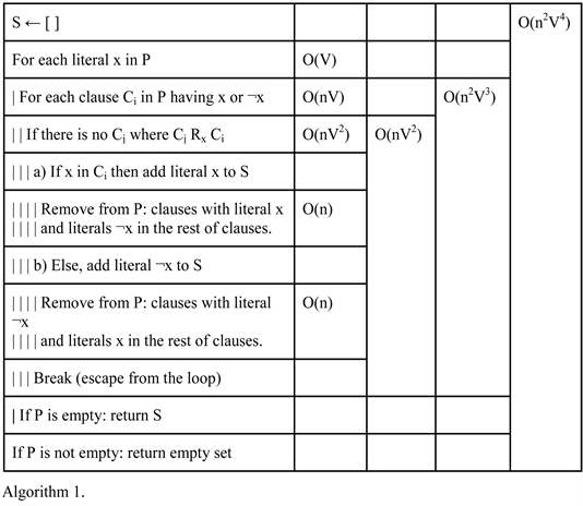
If the result of Algorithm 1 is the empty set, then if the input is a product of clauses it returns that the formula is unsatisfiable, while if the input is the union of minterms the empty set means that the formula is a tautology.

Examples:

In the following tables Table 1 and Table 2 we will analyze the formula:

(x + y + z + t)(x + ¬y + z)(x + y + z)(¬x + ¬y + z)(¬x + z + t)(¬x + y + z + u)

while in the tables Table 3 and Table 4 we will study:

(x + y + z)(¬x + z + ¬t)(x + ¬y + t)(x + ¬y + ¬t)(y + z + t)

Table 1. Example from (x + y + z + t)(x + ¬y + z)(x + y + z)(¬x + ¬y + z)(¬x + z + t)(¬x + y + z + u) = 1.

Table 2. Example from (x + y + z + t)(x + ¬y + z)(x + y + z)(¬x + ¬y + z)(¬x + z + t)(¬x + y + z + u) = 1.

Table 3. Example from (x + y + z)(¬x + z + ¬t)(x + ¬y + t)(x + ¬y + ¬t)(y + z + t) = 1.

Table 4. Example from (x + y + z)(¬x + z + ¬t)(x + ¬y + t)(x + ¬y + ¬t)(y + z + t) = 1.

Thesis. Algorithm 1 works well for formulae where literals do not change sign in the same clause.

COR: If thesis is true, Method 1 works with n-queens problem [Annex 8].

COR: For n queens algorithm is DTIME ~O(n¹⁴)

Dem. variables V~O(n²), clauses x ~O(n³)

DTIME (SAT) ~O(x²V⁴))

DTIME (n-queens) ~O(n^2·3+2·4) = O(n¹⁴)

3.2. Method 2

Based on our understanding of how the method 1 works, it can be versioned for a Turing machine whose cursor is not sequential, but random: that is, it can be used to work with machines that look a bit more like today’s computers.

To do this, we create a data structure that will help us predict which literals are likely to be avoided when a valid minterm is found. That is, the algorithm will end up generating the structure that we will use later to find various cases.

So we will use a new operator that will be applied on each pair of clauses:

${\text{A/}}_{\text{x}}\text{B}=\left\{\neg \text{z}|\text{z}\in \text{A}\wedge \text{Z}\notin \text{B}\wedge \text{z}\ne \text{x}\wedge \text{z}\ne \neg \text{x}\right\}$

$\text{A}:\text{B}=\left\{\text{x}|\text{x}\in \text{A}\wedge \neg \text{x}\in \text{B}\vee \neg \text{x}\in \text{A}\wedge \text{x}\in \text{B}\right\}$

$\text{A}\sim \text{B}=\{(\text{A}:\text{B},\text{A}{/}_{\text{A}:\text{B}}\text{B})\leftarrow |\text{A}:\text{B}|=\text{1}}$

Examples:

{1, 2, 3, −4}~ {1, 2, 4} = (4, {−3})

{3, −4} ~ {1, 2, 4} = (4, {−3})

{1, 2, 4} ~ {1, 2, 3, −4} = (4, Ø)

{1, 2, 3, −4}~ {−1, 2, 4} = Ø

{1, 2, 3, −4}~ {−1, 2} = (1, {−3, 4})

Another possible representation that can be chosen considering certain abuses of notation would be to use Boolean expressions:

(x + y + z + ¬ t) ~ (x + y + t) = (t, ¬z)

(z + ¬ t) ~ (x + y + t) = (t, ¬z)

(x + y + t) ~ (x + y + z + ¬ t) = (t, 1)

(x + y + z + ¬ t) ~ (¬ x + y + t) = Ø

(x + y + z + ¬ t) ~ (¬ x + y) = (x, ¬z·t)

This operator is the one that will allow us to go through the whole list of clauses and indexes to keep them updated.

Algorithm 2.1 Preparation of clauses to extract minterms efficiently.

Input: P = set of clauses; Each clause a set of boolean literals.

Output: = list of clauses and indexes; the indexes is a dictionary whose keys are the literals of the associated clause and the value mapping each key is a boolean function that triggers the prohibition to use that literal of the clause.

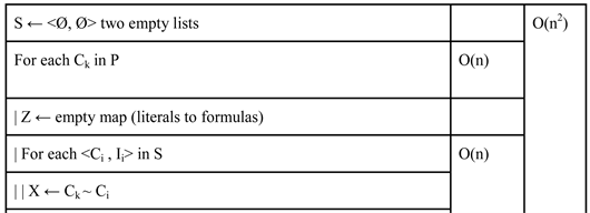
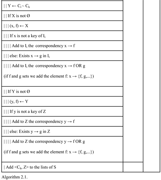
Once the two lists have been generated, the following algorithm must be applied to extract the k-th minterm:

Algorithm 2.2.

Input: S = , integer k

Output: M, minterm where ∏M = 1 → ∏C =1 or not if it were not possible.

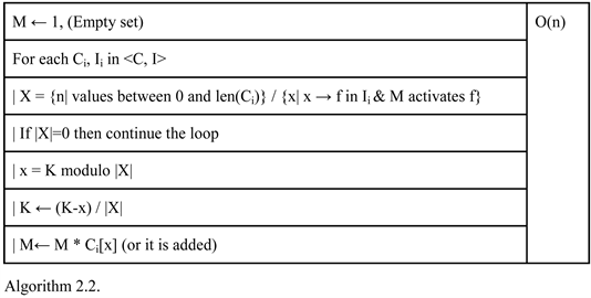
To understand Algorithm 2.2 the term “A activates B” has been used, it is understood that if A is a minterm and B a Boolean function then “A activates B” if A → B; i.e. A is a sufficient solution of B.

The following examples will be used to examine Algorithm 2.2.

Example 1.

In Table 5 we see which conditions must be fulfilled for the literals of each clause not to be chosen. For example, if q = 1 then clause 1 does not support the literal ¬p. Note how if the solution incorporates sp = 1 then clause 3 will not give a solution or that if the solution incorporates q = 0 then clause 4 won’t do it either.

So we will execute Algorithm 2.2 in Table 6.

In clause 2 r is deactivated because ¬s was chosen in clause 0, and q because ¬p. So, is it enough to finish the algorithm? We have to consider that clause 2 probably has more information than the rest in the case K = 0. Under an indexing there is an ideal order which is fixed to get a solution. So, if it is so, the clauses that succumb to an exception need to be put at the beginning.

That is why we will consider varying Algorithm 2.2 by permuting some clauses as shown in Table 7.

After executing the step in Table 7, we can continue permuting in Table 8 and Table 9.

At this point, in Table 10, we notice that clause 2 cannot be moved again: so it is enough to understand that the formula has no solution.

Table 5. Example of a formula without solution.

Table 6. Studying Table 5 in case K = 0 (the first literal in each clause if possible).

Table 7. Permuting Table 6 in case K = 0.

Table 8. Step from Table 7 in case K = 0.

Table 9. Step from Table 8 in case K = 0.

Table 10. Step from Table 9 in case K = 0.

This algorithm can be called Algorithm 2.3, that is an iterative version of Algorithm 2.2.

Example 2. Table 11 will be the same example 1 but without clause 3. That is for incorporating a solution.

From Table 11 we will study how Algorithm 2.2 works in Table 12 and Algorithm 2.3 in Table 13.

So from Table 13 we see now the solution is: ¬r·p·s·q.

Example 3.

For the next example in Table 14 we will consider a formula of 3 literals.

Notice that clause 0 can be substituted by (x + z) or clause 2 by (x + ¬y). So after using Algorithm 2.2 for different K.

0: xz, 1: zx, 2: x¬ty, 3: z¬y, 4: xz, 5: zx...

We get these minimal solutions: xz + xy¬t + ¬yz.

Thesis. Algorithm 2.3 only succumbs to an exception when the formula is unsatisfiable.

COR: If the thesis is true, Method 2 solves any boolean formula in polynomial time.

Table 11. Example of formula with a solution.

Table 12. Studying Table 11 in case K = 0.

Table 13. Permuting Table 12 in case K = 0.

Table 14. Example with a formula of 3 literals.

3.3. Method 3

It is possible to speak of a third method whose complexity is lower, provided that it takes advantage of having several machines running in parallel. Using matrix notation, n machines on an input of n clauses can distribute the work of multiplying the matrix by itself and go from having a cost of O (n² log n) to being O (n log n) for large inputs.

To do this, the following rules must be available:

1) Two clauses of size n and m generate a submatrix of 1’s of nxm.

2) Every literal i and j that are opposites becomes 0 in (i, j).

3) Every literal i and j that are the same becomes 0 in k ≠ i (i, k) and k ≠ j (k, j).

In this way a matrix is formed as in Table 15 with the submatrices relating all clauses to themselves to form a square matrix of size mxm where m is the sum of

Table 15. Matrix T⁰.

all literals along the input, or the product of the number of literals per clause times the number of clauses if it was the same.

The matrix product consists of calculating the scalar product of row and column and returning 1 if the result is greater than or equal to n; n is the number of clauses.

When the matrix multiplied in this way with itself gives the same matrix we will say that it has reached a Noetherian ideal, and if it maintains the main diagonal then we will proceed to find a k-th solution. To find the k-th solution we only have to choose a pair of clauses whose submatrix has more than one 1 and we select only one 1, then we calculate its noetherian ideal and if the result is 0 then it was inconsistent, if on the contrary we repeat the procedure until the matrix reflects a single minterm.

For the next formula.

$T_{ij}^{m+1}=T_{ij}^m\wedge \left[{\displaystyle {\sum }_{k=0}^{k=m}{T}_{ik}^m\cdot T_{kj}^m}\right]\ge n$

$T_{12}^0\wedge \left[T_{11}^0\cdot T_{12}^0+T_{12}^0\cdot T_{22}^0+T_{13}^0\cdot T_{32}^0\right]\ge 3$

$\begin{array}{l}\left(\begin{array}{ccc}0& 1& 1\\ 1& 0& 1\\ 1& 1& 0\end{array}\right)\wedge [\left(\begin{array}{ccc}1& 0& 0\\ 0& 1& 0\\ 0& 0& 1\end{array}\right)\left(\begin{array}{ccc}0& 1& 1\\ 1& 0& 1\\ 1& 1& 0\end{array}\right)+\left(\begin{array}{ccc}0& 1& 1\\ 1& 0& 1\\ 1& 1& 0\end{array}\right)\left(\begin{array}{ccc}1& 0& 0\\ 0& 1& 0\\ 0& 0& 1\end{array}\right)\\ +\left(\begin{array}{ccc}0& 0& 1\\ 0& 1& 0\\ 1& 0& 0\end{array}\right)\left(\begin{array}{ccc}1& 0& 0\\ 0& 0& 0\\ 0& 0& 1\end{array}\right)]\ge 3\end{array}$

$\left(\begin{array}{ccc}0& 1& 1\\ 1& 0& 1\\ 1& 1& 0\end{array}\right)\wedge [\left(\begin{array}{ccc}0& 1& 1\\ 1& 0& 1\\ 1& 1& 0\end{array}\right)+\left(\begin{array}{ccc}0& 1& 1\\ 1& 0& 1\\ 1& 1& 0\end{array}\right)+\left(\begin{array}{ccc}0& 0& 1\\ 0& 0& 0\\ 1& 0& 0\end{array}\right)]\ge 3$

$\left(\begin{array}{ccc}0& 1& 1\\ 1& 0& 1\\ 1& 1& 0\end{array}\right)\wedge \left(\begin{array}{ccc}0& 0& 1\\ 0& 0& 0\\ 1& 0& 0\end{array}\right)=\left(\begin{array}{ccc}0& 0& 1\\ 0& 0& 0\\ 1& 0& 0\end{array}\right)=\neg \text{x}\wedge \neg \text{z}\vee \text{x}\wedge \text{z}$

What this algorithm should induce us is that it is still possible to find methods that on the most powerful machines can give us more efficient results than the quadratic one.

It is easy to see this algorithm will work because this little lemma:

$A_i\left(A_i-1\right)=0\Rightarrow {\displaystyle \prod A_i}=u\left(-n+{\displaystyle \sum A_i}\right)$, where u(x) = 1 iff x is not negative, else 0.

Considering a matrix is formed by subtables, each table with only one solution is enough to be a sufficient condition to ensure the satisfiability of the complete formula under a Noetherian ideal, as it is exposed in Table 16, because every solution will get catched.

So after finding a solution if there is noone f is unsatisfiable.

4. Correctness and Efficiency of Methods

The engine that solves methods 1 and 2 are the same, and the motivation that justifies the results of methods 2 and 3 are also based on the same. The first method expects an input whose literals in each clause do not complicate the results. The second method, however, works optimally if the clauses are available in the right order, which can be evaluated by pre-calculating their structure. In fact, the superstructure of method 3, even if it incorporates new solutions in its ideal, these will be eliminated by collapsing them to the search for a single case. Therefore, at least in method 3, we can be absolutely certain that the method works.

In all three methods, if the input of the algorithm is a set of clauses the result is a minterm that solves the formula, while if it is a set of minterms the result is a clause that contradicts the formula. So the objective is to calculate a term not neutral after applying the distributive operation of sums and products.

Method 1 works on a sequential machine, while method 2 works on a random access machine. Method 3 works on a random access machine, and is easily distributable on machines working in parallel.

The Outer Loop of Algorithm 1

Attention should be drawn to the outer loop of the algorithm, as it traverses the variables of the formula; which must be a constant value with respect to the size of the input. It is still possible that for some problems the number of variables may be made variable, in which case it should be studied to what extent the most likely performance of the algorithm can be studied.

Table 16. Relationship between the original formula and the Noetherian Ideal of its matrix.

To begin with, the outer loop runs through all variables as long as it finds any pair of clauses containing both affirmed and negated variables. So if only one contains it, it will automatically correspond to the elimination of that clause. That is, the loop expects to delete clauses as it recognises variables. So if the variable expression were larger than the clause expression, the loop could be reinterpreted as O (n³V³) where n is the number of clauses and V the number of variables. Although, essentially, in reality the algorithm is quadratic.

5. Discussions

After reading the conclusions of Section 4, it follows that SAT is in P and moreover it is not transcomputational. Furthermore, it follows that there is polynomial resolution also in the n-queens problem by taking the number of queens as a variable value [Annex 8]. If we combine this result with the Levin-Cook theorem, as well as with Fagin’s papers [10] or Karp’s conclusions [11], it follows that the class NP = P because they believe they have proved that SAT is part of NP-completeness, which means that if this problem is solvable in polynomial time then any NP-problem will be solvable in polynomial time.

However, does that mean that any cryptographic algorithm that is expressed as an NDTM configuration will quickly have an TM that decrypts it? If so, why is there no library that implements the formula posed by Cook’s theorem?

On the other hand, Fagin considers that an NDTM can be expressed through second-order logic; knowing that PROLOG is an example of a programming language that can work under these conditions. However, it can be proved that if the formulas could be expressed in Horn clauses [12], then the resolution would be in P time.

Now, isn’t there some equivalence between a product of clauses and a product of Horn clauses? Well, there is a probabilistic equivalence that makes the problem reduce to class R, which is the class of problems that are solved under high probability. That is, if cryptographic problems could be solved probabilistically high, as this reference states, then it would not matter that their resolution is exponential in the worst case, because from a practical point of view it would be easy to break most cryptographic systems. In fact, from the way the Annex 7 is developed, we see that equivalence between clauses is a trivial process, which anyone could try. However, there is no library in PROLOG, or in CAML, that develops any problem. The reason is that the world designed from a formal logical theory is not comparable in intelligibility with the operations that take place within an unrestricted grammar. Second-order logic will not help predict what is decidable, as Turing claimed.

On the other hand, in Matiyasevich’s words [13], Julia Robinson failed to find a polynomial formula to replace an exponential, but she found sufficient conditions. That is to say, given a formula expressed exponentially, as corresponds to the limit established by Turing as the number of demonstrations that an a-TM needs to simulate a c-TM, it is possible to find a polynomial expression that represents the same limit. So formally, there will always be a polynomial coordinate linking NP with P, as a corollary. However, neither has it been seen that the Matiyasevich formulation was developed to represent any diophantine equation. Note, for example, that elliptic equations are amenable to representation within the polynomial coordinate, but there is no technology to develop it. Another formalism?

6. Discrepancies

A recurring theme in my rebuttals will be to say that we do not see libraries, code, structures, etc., created from these theoretical concepts. However, the reason we do not see them is not because the statements do not link to technological reality, but because the way the statements are answered is incompatible with the technology. That is, with a different technology the demonstrations will go hand in hand.

So we need a more correct philosophy, namely more rigorous than mathematical formalisms. And Cook’s theorem is perfect to understand what I mean.

6.1. Refutation of Cook’s Theorem and Relatives

Cook’s theorem tells us that given a configuration of a TM that is classified as an NP-problem (it ends up in two possible states Q_Y or Q_N after a number of steps no greater than a polynomial expression whose variable is the size of the input) this configuration can be transformed into a product expression of disjunctions of logical literals. Where a literal is an affirmed or negated variable, and a variable is a value between true or false.

The formalism we are going to focus on is the fact that we do not have an exact expression of how long it will take for NDTM to determine the final state. At all times we will have an expression in [2] of the form p(n), where n is not the input, but the size of the input and where p is a polynomial function that can be determined, as long as it is an expression of maxima. That is, the intended value is always less than p(n).

But can we attribute to a NDTM configuration a polynomial expression from the size of the input that delimits the termination time? No. In fact, a bound less than infinity cannot be assured, as Turing’s conclusion established by decidability [9], so a polynomial bound is even more impossible.

That is why Cook’s theorem is not constructible, the input to be passed to the machine that generates the input to SAT is also a polynomial expression with respect to the size of the input.

Given a computer security protocol based on a one-way function, we configure a NDTM to evaluate whether a certificate results in the value given in the input and we have a maximum limitation on the size of the certificate to establish that it is an NP problem. That is, as with the halt algorithm, the existence of a correspondence does not imply that the configuration can actually be constructed; the correspondence may be a formalism that does not fit with a particular TM configuration. This paradox is further developed in the annexes [Annex 3].

6.2. The Complementary of an NP Problem Should Not Be a Difficult Concept to Calculate

It is striking what Fagin does when he develops the idea of taking the expression of a problem and calculating its complementary [10]. When a language is expressed in such a way that we want to determine its complementary, here we see how Cook and Fagin provide us with comments that are very lacking in rigor: how do we determine the complementary of a problem?

On the one hand, we see how Cook tells us that the complementary of the SAT problem is to determine whether a formula is a tautology. In the appendices we see that the tautology is trivially SAT [Annex 5], so hasn’t Cook noticed?

Fagin, however, is more mystical when it comes to determining a complementary. One would expect that if a set of inputs (such as prime numbers) we want to extract its complementary (such as composite numbers) then there must be a unique correspondence in a clear-cut way. However, the real numbers are contained within the complementary of the naturals, which encompasses the prime numbers, so presupposing that composite numbers is the complementary of the primes forces us to reject the real numbers as numbers.

Even so, in the annexes [Annex 4] I provide an objective mechanism for determining the complementary of a problem; specifically an NP-co according to Fagin. The resolution of that annex tells us that its complementary is an NP, so according to Fagin’s theorem 15 in [10] coNP = NP.

The problem with this statement is that it is easy to determine the complementary of SAT. However, if we create an NP-problem full of very heterogeneous variables and domains, the definition of the complementary can lead us to structures that could be defined in a non-rigorous way. That is, it is possible to define NP-problems where co-NPs are not decidable.

For example,

1) calculate the result of a diophantine equation where the variables are bounded by a fixed value.

2) solve Post’s problem for inputs not greater than a certain length.

3) determine the halt of algorithms that do not exceed a certain computation time.

It must be understood that the existence of NP-co contradicts the existence of complementary NPs.

6.3. Formalism Cannot Statically Represent a Dynamic Problem

When a problem is posed, the input x corresponds to a resolution of acceptance or rejection. If there were a mechanism to speed up the decision process in the decision making of the possible bifurcations the same decision process is demonstrated in the annexes [Annex 6] which is actually another way of expressing the input.

The annex shows that it is not possible to work with a static decision maker that works for all inputs, but that the decision maker is specific to each input. This leads to the fact that it is not possible to work with NP-co problems.

6.4. Fagin Works with Second-Order Logic and Forgets Horn’s Clauses

Another striking detail is how easy it is to convert a second-order logic (SO) problem that is very close to Horn clauses. In the appendix [Annex 7] it is shown that for practical purposes, not so much formal ones, Horn clauses simulate any SO formula as do current algorithms that calculate the primality of a number: with all the probabilistic precision we want.

That is, Fagin claims in his paper [10] that second-order logical formalisms are equivalent to the NP class. That belief would lead us to believe that for practically any NP problem we will always have a representation that can be easily validated in polynomial time and that, with all the probability we need, will end up returning a practical result.

However, nobody uses PROLOG or CAML to crack security protocols. It is a practical absurdity. Fagin has not helped at all to predict how technology works with this strange dogma.

6.5. By Mathematical Formalisms We Will Always Say NP = P

In an unappealable way, we see in the appendices [Annex 9] that Julia Robinson found a way to express any expression that uses the variable in the exponential to put it in the base of the power function. However, Matiyasevich correctly explained how this result should be interpreted: Julia Robinson failed in the constructive proof, but not in the formalism of the necessary condition.

That is, a value needs to be incorporated which has not been established and which connects the problem to the transcomputational. However, formally one could already say, if a TM were defined with mathematical formalisms, that NP = P. For that would be the most accurate and, at the same time, the most useless for engineering.

7. Conclusions

When Cantor presented his idea that there are many infinites, Poincaré considered these ideas to be a disease for mathematics. Cantor’s formalisms led to the development of differential equations, and these led to the development of the theory of relativity, among other things. Therefore, even if formalisms are a looser mathematics, this does not mean that they are of no practical use.

Just as we have shown that mathematical formalisms cannot describe the complexity of the notation of a TM, what they can define allows us to work under the assumption that NP = P. As long as the inputs comply with a certain continuity that does not exploit the lack of rigor of the formal version of the TM. However, when we work with cryptographic data, the inputs will be too variable to assert that the same thing will continue to be true.

That is, depending on what you are going to use the Turing machine for, it is better to define it in one way or another. And that is the meaning of this essay: mathematical formalisms are neither better nor worse than constructivism. They develop in different areas. And after reading this essay one has to accept that any problem that is polynomially reduced constructively with SAT will have a polynomial, non-transcomputational and probably trivial resolution.

The Conspiracy Theorists

Finally, it would seem legitimate, at least, to consider whether it is not possible that all this technology was already known and expressly hidden. What is in it for the various authors who claimed to be unaware of this possibility, as well as university professors, lecturers, etc. What is in it for all these huge numbers of people repeating something they knew was nothing but propaganda? One has to think of influencers and foundations offering rewards, can one therefore expect that all the rewards were placed in the hope that no one could solve such problems? If so, it would confirm the belief that this technology is really a milestone for technology.

One has to think of so many blog articles and Youtube videos that have been written under the assumption of the non-existence of the technology in this test, and that they could become obsolete as soon as someone would figure out how to solve these puzzles.

Moreover, how could companies that depend on delivering breakthrough results and depend on operational research to the point of seeing their revenues multiply by reducing management costs on any of the 300 problems associated with this article pretend to ignore the existence of this technology? Is there a two-tier capitalism, as in companies that have a right to know about the existence of this technology and companies that don’t?

The same has happened with the pharmaceutical industry or all governments in general when it comes to COVID: when it comes to creating vaccines, storing and distributing them, it could well be done in the most efficient way by a very close mathematical problem. However, admitting that such a technology already exists, where would that put the executive branch—wasn’t it said that we need a democratically imposed policy by a human being to choose how best to run the administration? If in the end a mathematical model is the dictator telling us what is the most efficient resolution, then is that our conspiracy, that they will not want to admit the existence of this technology because it might displace the executive from its beneficent role?

But not only that, whenever there is an innovation that brings about a radical change in thinking, the more senior people tend to try to crush the newer ones in the field. This unionization could be multiplied if a person who is not part of the official world ends up solving a major problem; as if it had happened overnight, because nobody knew about it until that moment. It is clear that the refusals could reach the point where peers will respond in a highly dastardly and overt manner. All for the sake of maintaining the guild and the corporation.

So we are left with the hacker world. Did they have access to this technology? What is really undeniable is that if this publication does not reach the official eyes of all, that world will benefit the most of all, and then the only reason why this technology will pose a security risk is because those working in these fields have decided to do so.

9. Appendix

9.1. Annex 1. Factoring Is P-Reducible to SAT

We will give an example of how some protocols are susceptible to find a SAT formula. The purpose of this annex is to encourage cryptographers to better select their security protocols.

To begin with, let us define a logical operation of Boolean propositions:

(A|B|C): returns true if one and only one of the propositions is true.

Therefore:

(A|B|C) = A¬B¬C + ¬AB¬C + A¬B¬C.

Likewise, it is easy to deduce that:

(A|B|C) = (¬A + ¬B + ¬C)(A + ¬B + ¬C)(¬A + B + ¬C)(¬A + ¬B + C)(A + B + C)

Corollary: A formula written with operators | and products is proportional in space to a formula written with or and products.

Now we incorporate the following theorem:

Theorem: (¬A|AB|Z1)(¬B|AB|Z2)(Z1|Z2|¬A XOR B) = 1, given A, B Boolean propositions.

What the above theorem tells us is that it is equivalent to work with problems within SAT than with problems expressed with | and products. Therefore, when we see a well-formed formula that uses XOR operators we can trivially transform it to an expression of products of | or products of or easily.

Given a natural number we are interested in knowing which two natural numbers multiplied together give the same number. It is possible to incorporate the restriction that both be greater than 1, but here we will simply study how easy it is to find the SAT expression constructively.

N = A × B, we ask ourselves about the values of A and B

$\begin{array}{l}A={\displaystyle {\sum }_{i=0}^n{a}_i{2}^i}\\ B={\displaystyle {\sum }_{i=0}^n{b}_i{2}^i}\\ N={\displaystyle {\sum }_{i=0}^n{h}_i{2}^i}\end{array}$

To relate the coefficients of the unknowns to the expected result, we create a table that will help us to know how the logic gates will be organized.

In the following Table, I will use three types of logic gates:

Gate A takes the top value u and the left value I as inputs and returns right u XOR I, while returning down u AND I.

Gate + takes the value of up and returns down and the value of left returns right.

Gate L takes the value from below and returns it to the right.

In Table 17 you can see how to connect the gates.

We note that the number of gates A is quadratic with respect to the input size. When the remaining gates have no impact on the complexity of the formula.

Therefore the factorisation of numbers is polynomially reducible to SAT constructively.

Table 17. Distribution of the gates.

9.2. Annex 2. Strict Implication

According to [14]. Given A, B propositions of logic are given: (A → B) OR (B → A) = True se can see its demonstration in Table 18.

As a corollary it follows that it will always be true: (A → ¬A) OR (¬A → A), from which it follows that the implication is not very similar to a precedence operator. That is, it does not work very well to say that the implicant is guaranteed by the implicant.

9.3. Annex 3. Formalisms Do Not Fit Transformation Operations

We are going to have a Turing machine that transforms states over time thanks to a configuration σ. The logical formalism tells us that Q_a Q_b if and only if there exists an integer K where Q_{a, k} → Q_{b, k+1}, where → is the logical implicator. Moreover we know that the fact that Q_a Q_b in the Turing machine implies a that the transition (a, b) is described in σ. Being a and b two indices to complete states of a Turing machine, not only its register.

So we start from a Turing machine that intends to solve a problem that will end in two possible final states: Q_{Y, T} or Q_{N, T} at some T for each input.

1) We define Q_{z, k} a state through which the input to which we submit the machine in time k does not pass and which leads to the rejection Q_{N, k+1} directly.

2) (z, N) is transition described in σ according to 1.

3) For all k: Q_{z, k} → Q_{N, k+1} [It follows from 2 and 1, leads to rejection].

4) (Q_{z, k} → Q_{Y, k+1}) OR (Q_{Y, k+1} → Q_{z, k}) [theorem to be taken from Annex 2].

a) Sup Q_{z, k} → Q_{Y, k+1}

b) Formally we deduce that Q_{z, k} implies two different states in a deterministic machine.

Both Q_{Y, k+1} and Q_{N, k+1}.

5) Q_{Y, k+1} → Q_{z, k} [It follows from the previous branch, by contradiction].

6) Q_{Y, k+1} → Q_{N, k+1} [Combining steps 3 and 5].

7) So if a state is recognised it is also not recognised at the same time.

Therefore the formalisms are too lax to represent machines.

9.4. Annex 4. The Complementary of SAT Is SAT

Thus, every problem that reduces to SAT has as its complementary an NP.

Table 18. Demonstration (A → B) OR (B → A) is a Theorem.

When determining the complementary of a language L, we will say that if w є L then LC is the complementary and ¬(w є LC). So if we say that L belongs to a class that is closed by its complementary then LC will also belong to the class.

We start from the expression we use to represent an entry in SAT

SAT: Ǝx_i: x_i є Boolean → f(x_i) = 1

SAT^c: ¬(Ǝx_i: x_i є Boolean → f(x_i) = 1)

To determine the complementary we must first extract the quantifier

SAT^c: x_i: ¬(x_i є Boolean → f(x_i) = 1)

The next is to negate the implicator

SAT^c: x_i: x_i є Boolean & ¬( f(x_i) = 1)

It only remains to recognise that if the variables are Boolean and a Boolean formula is negated then the result is the complementary:

SAT^c: x_i: x_i є Boolean & f(x_i) = 0.

Therefore, SAT^c consists exactly of:

1) Determine if the variables in the input are boolean. If they are not, return Q_N.

2) Assign to R the result of SAT for that input.

3) If R is Q_Y then return Q_N; otherwise return Q_Y.

As can be seen trivially SAT^c reduces trivially from SAT.

9.5. Annex 5. Tautology Is SAT

We are going to show that finding the tautology of an expression is finding SAT. To do this we are going to do a series of automatic and equivalent transformations:

SAT: Ǝx_i: x_i є Boolean → f(x_i) = 1.

TAU: x_i: x_i є Boolean → f(x_i) = 1

We will develop TAU to see how we reduce it from SAT by the double negation theorem:

TAU: ¬¬(x_i: x_i є Boolean → f(x_i) = 1)

TAU: ¬Ǝx_i: ¬(x_i є Boolean → f(x_i) = 1)

TAU: ¬Ǝx_i: x_i є Boolean & ¬(f(x_i) = 1)

The expression of f is Boolean and the TAU problem works with Booleans, so the complementary will be the Boolean complementary:

TAU: ¬(Ǝx_i: x_i є Boolean & ¬f(x_i) = 1)

TAU is to ensure that we will not find boolean variables that return 1 in the complementary boolean expression put in the input. However, as can be seen in the appendix, the Boolean complementary of SAT constructively forms part of SAT and reduces polynomially. So ¬f = f^c.

TAU : ¬(Ǝx_i: x_i є Boolean & f^c(x_i) = 1)

That is,

1) We determine what the complementary function of the input is [Annex 1].

2) We assign to R the final state of SAT over the complementary function.

3) If R = Q_Y, then TAU must end in Q_N. If R = Q_N, then TAU ends in Q_Y.

9.6. Annex 6. When NP-Complete Problems Are Not Possible

Let us start from an expression formulated with diophantine equations, whose variables are bounded by a constant K:

Ǝx_i: x_i < K → D(x_i) = 0. (1)

We ask ourselves if it is possible to find some integers that satisfy a diophantine equation. If we make a simple transformation, we can transform Eq1 into another equation by converting the constant into a variable:

Ǝx_i, Ǝz: x_i < z → D(x_i) = 0. (2)

Equation (1) covers the whole spectrum of NP-problems according to Cook, since it is not the concern of formalists to ensure the existence of a machine, but that its variables are bounded so that there is a verification in polynomial time. However, Equation (2) corresponds to the spectrum of all TMs, and is the set of all enumerable problems, because for each diophantine equation an additional variable can always be defined a posteriori whose value is greater than that of all the variables without any change in the number of solutions, nor any complication in computing it.

However, we can change Equation (2) for another equation which we will see is equivalent:

Ǝx_i, Ǝz: x_i < K < z < 2^K → D(x _i) = 0 (3)

At this point we have defined the new variable z as having to be at a value between a value supremum to all variables and its exponential of two. This can also be assumed, for example:

z = Σx_i²

That is, without having to define a K value as a constant, a diophantine equation can be extended to have a polynomial coordinate with respect to the values of the variables that would solve the input.

Let’s say that z is the certificate that an NDTM needs to give a solution to a diophantine equation D. So z = f(D), and it is given that the number of decisions that must be made in the machine to make it deterministic will be K. So the question is whether the function f that creates the certificate for any diophantine equation is decidable.

We must understand that D has a constant value with respect to the size of the input, so if f exists then z will also be a constant value.

Ǝx_i: x_i < K < f(D) < 2^K → D(x_i) = 0 (4)

And this leads us to the fact that Equation (4) is equivalent to Equation (2) and Equation (1) at the same time. So when in Equation (2) or Equation (1) a correspondence is established between the configuration of a Turing machine and its input-independent certificate then that leads us to an inconsistency.

Corollary 1: The certificate is an expression of the input.

Corollary 2: NP-complete problems are not possible.

Dem. An NP-complete implies that solving that problem independently of the input directly generates the certificate. This is inconsistent.

Corollary 3: There can be specific MT definitions for which NP-co exists.

Dem. An MT with restricted inputs does not generate the merging of Equation (2) and Equation (4), so an MT could be defined from a set of constraints that the input will have and not cause the inconsistency.

9.7. Annex 7. There Is a Formula in Horn Clauses Practically Equal to Any Fbf

Under a practical computer science philosophy, it is possible to create algorithms that are sufficiently accurate to work well in average cases [15]. An example of this will be presented here: For any probability value p > 0 and f second-order logical formula, we will say that there exists a formula h expressed in Horn clauses whose satisfaction will coincide with f under probability greater than p.

To achieve this we will start from an expression of the form 3-SAT for simplicity, where all the clauses are formed by the sum of three literals (affirmed or negated propositions) and that multiplied gives us the formula to be satisfied.

The exercise to be carried out in this annex will be to establish a link between 3-SAT and HORN. To do so, we will recognise all the clauses that are in SAT and cannot be in HORN, these are of the form:

1) (x1 + x2 + x3)

2) (x1 + x2 + ¬x3)

3) (x1 + x2)

In the sense that there must not be more than one asserted literal. So we collect all the variables V that have an asserted literal in these clauses.

We start from the clauses of R a copy of the clauses of SAT and determine a k large enough to comply:

$p>{\left(\frac{2^k-1}{2^k}\right)}^{\left|V\right|}$

where |V| is the number of variables and p is the value set as the minimum probability that HORN will solve SAT.

For each of these variables V we proceed as follows:

1) K new variables associated with V are created, called V₁, ···, V_k.

2) The clauses (¬V + ¬V_i) for each i between 1 and k are incorporated into the formula R.

3) For each clause where V appears in R, V is replaced by ¬V_i, for each i, proceeding to version the clause for each i from 1 to k.

The result R will be an expression of HORN clauses to which spurious solutions have been added which, in proportion to the large number of valid solutions, will not represent more faults than you want to assume.

If the algorithm is well programmed, the size of the input will have been extended by no more than O (k²).

9.8. Annex 8. Transformation of the n-Queens into SAT

The n-queens problem consists in the fact that we have a board of nxn and we must place n queens on it without any of them threatening each other according to the rules of chess.

The peculiarity of the n-queens problem is that as n increases, the number of variables in the formula will increase. However, since our methods work independently of the number of variables because it is not a formalism, this will not be relevant.

To determine how large the input will be we can recognise a quadratic number of variables with respect to the number of queens, where each variable will recognise four coordinates: (f, c, a, b). Where f is the row number, c is the column number, a is the secondary diagonal number and b is the main diagonal number.

If we choose an example representation it would be as shown in Table 19.

It can be seen that from the row and column coordinates the values of a and b can be deduced. Trivially: a = f + c − 1; b = f − c + n

When it comes to creating the clauses, we will have two types: on the one hand there will be the clauses formed by the restriction that they must not threaten each other

1) By rows: (¬Tfcab + ¬Tfc'a'b') O(n³) clauses are incorporated.

2) By columns: (¬Tfcab + ¬Tf'ca'b') O(n³) clauses are inserted

3) By diagonal a: (¬Tfcab + ¬Tf'c'ab') O(n³) clauses are inserted

4) By diagonal b: (¬Tfcab + ¬Tf'c'a'b) O(n³) clauses are incorporated.

With these clauses we avoid putting extra checkers, but at least we have to count n checkers. To impose the restriction of placing n draughts, the following clauses are incorporated: (Tf1a1b1 + ··· + Tfnanbn). n clauses are incorporated.

Therefore, all conditions covered we observe that the n-queens problem is solvable by means of an input with O (n³) clauses. Partially incorporating the solution of the problem will not lead to an increase in complexity.

Table 19. Example of naming the positions in the n-Queens.

9.9. Annex 9. Every Exponential Expression Has a Polynomial Expression

In this annex I will demonstrate that, without using a constructivist philosophy of the processes of mathematical demonstrations, every exponential expression has a polynomial expression, so the maximum bound is polynomial in both space and time.

Alan Turing showed that a NDTM (choice TM in [9]) requires a cost O(2^x) with x the size of the input to simulate a deterministic TM (automatic TM).

However, given the work of Julia Robinson [13], the expression 2^x = t can be expressed by diophantine equations with polynomial expressions of the form t~O(x^k) for k constant, independent of x.

One must work with a sufficiently large M so that it satisfies: M > 2·x·2^x , i.e. is there a sufficiently large number that meets this requirement? Considering that x is less than infinity there will always be such a number, so formally NP = P. However, M must be determined from a supreme input size, so since there will always be inputs whose size is larger than M then constructively equality is not assured.

On the other hand, working with large M means that the constant by which the polynomial expression multiplies will end up being a transcomputational number. So this would not be a practicable statement in principle either. Which is another example of why formalisms do not fit the requirements of machines.

Conflicts of Interest

The authors declare no conflicts of interest regarding the publication of this paper.

References

[1]	Cook, S. (2003) The Importance of the P versus NP Question. Journal of the ACM, 50, 27-29. https://doi.org/10.1145/602382.602398
[2]	Garey, M.R. and Johnson, D.S. (2009) Computers and Intractability: A Guide to the Theory of NP-Completeness. W.H. Freeman, New York.
[3]	Miles, W. (2011) “Bremermann’s Limit”.
[4]	NSA Press Releases & Statements (2012) National Cryptologic Museum Opens New Exhibit on Dr. John Nash.
[5]	Arora, S. and Barak, B. (2016) Computational Complexity. Cambridge University Press, Cambridge.
[6]	Dockrill, P. (2017) Anyone Can Win $1 Million by Solving This Wildly Complex Mathematical Chess Puzzle. https://www.sciencealert.com/if-you-like-chess-and-free-money-we-have-some-really-really-good-news
[7]	Popper, K. (1978) Three Worlds. The Tanner Lecture on Human Values. The University of Michigan, Ann Arbor.
[8]	Abdulla, P.A. and Jonsson, B. (1996) Verifying Programs with Unreliable Channels. Information and Computation, 127, 91-101. https://doi.org/10.1006/inco.1996.0053
[9]	Turing, A.M. (1937) On Computable Numbers, with an Application to the Entscheidungsproblem. Proceedings of the London Mathematical Society, S2-42, 230-265. https://doi.org/10.1112/plms/s2-42.1.230
[10]	Fagin, R. (1974) Generalized First-Order Spectra and Polynomial-Time Recognizable Sets. In: Society for Industrial and Applied Mathematics, Ed., Complexity of Computation, American Mathematical Society, Providence, 27-41.
[11]	Karp, R.M. (1972) Reducibility among Combinatorial Problems. In: Miller, R.E., Thatcher, J.W., Bohlinger, J.D., Eds., Complexity of Computer Computations, The IBM Research Symposia Series, Springer, Boston, 85-103. https://doi.org/10.1007/978-1-4684-2001-2_9
[12]	Dowling, W.F. and Gallier, J.H. (1984) Linear-Time Algorithms for Testing the Satisfiability of Propositional Horn Formulae. The Journal of Logic Programming, 1, 267-284. https://doi.org/10.1016/0743-1066(84)90014-1
[13]	Matijasevich, Y. (1992) My Collaboration with Julia Robinson. The Mathematical Intelligencer, 14, 38-45. https://doi.org/10.1007/BF03024472
[14]	Relevance Logic. https://plato.stanford.edu/archives/sum2009/entries/logic-relevance/
[15]	Spielman, D.A. and Teng, S. (2009) Smoothed Analysis: An Attempt to Explain the Behavior of Algorithms in Practice. Communications of the ACM, 52, 76-84. https://doi.org/10.1145/1562764.1562785