Tensor Robust Principal Component Analysis via Hybrid Truncation Norm ()

1. Introduction
Tensor is a multidimensional extension of matrix and an important data format, which can express the internal structure of more complex high-order data. In fact, tensor is also the natural form of high-dimensional and multi-way real-world data. For example, in the field of image processing [1], a color image is a 3-order tensor of height × weight × channel and a multispectral image is a 3-order tensor of height × weight × channel. Therefore, tensor analysis has important practical significance and application value in the fields of machine learning [2], computer vision [3], data mining [4], and so on. The tensor, we interest, is frequently low-rank, or approximately so [5] and hence has a much lower-dimensional structure. This has stimulated the problem of low rank tensor estimation and recovery, which has attracted great attention in many different fields. The classical principal component analysis (PCA) [6] is the most widely used method for data analysis and dimensionality reduction. For the data slightly damaged by small noise, it has the characteristics of high computational efficiency and powerful function. However, a major problem with principal component analysis is that it is easily affected by seriously damaged or bizarre observations, which are ubiquitous in real-world data. So far, many principal component analysis models [7] [8] have been proposed, but almost all of them have high computational cost.
RPCA is the first polynomial time algorithm with strong performance guarantee. Suppose that we are given an observed
, which can be decomposed as
, where
is low-rank and
is sparse. [6] shows that if the singular vector of
satisfies some incoherent conditions, such as
is low rank and
is sparse enough,
and
can be recovered accurately with high probability by solving the convex problem (1):
(1)
where
denotes the nuclear norm (sum of the singular values of
), and
denotes the
-norm (sum of the absolute values of all the entries of
). The parameter
is suggested to be set as
which works well in practice. In terms of algorithm, (1) can be solved by efficient algorithm, and the cost will not be much higher than PCA. This method and its generalization have been successfully applied to the fields of background modeling [9], subspace clustering [10], video compression sensing [11] and so on.
A major disadvantage of RPCA is that it can only process two-dimensional (matrix) data. However, real data is usually multi-dimensional in nature-the information is stored in multi-way arrays known as tensors [5]. To use RPCA, we must first convert the high-dimensional data into a matrix. However, such preprocessing usually leads to information loss, resulting in performance degradation. In order to alleviate this problem, a common method is to use the multidimensional structure of tensor data to deal with it.
In this paper, tensor robust principal component analysis (TRPCA) is studied in order to accurately recover the low rank tensor damaged by sparse noise. Suppose that we are given an observed
, which can be decomposed as
, where
is low-rank and
is sparse, and both components are of arbitrary magnitudes. Note that we do not know the locations of the nonzero elements of
, not even how many there are. Now we consider a similar problem to RPCA. This is the problem of tensor RPCA studied in this work.
It is not easy to generalize RPCA to tensor. The main problem of low rank tensor estimation is the definition of tensor rank [12]. At present, several definitions of tensor rank and its convex relaxation have been proposed, but each rank has its limitations. The CANDECOMP/PARAFAC (CP) rank of tensor [5] is defined as the minimum number of tensor rank 1 decomposition, which is NP-hard to calculate. Because of its unclear convex envelope, the recovery of low CP rank tensor is challenging [13]. A robust tensor CP decomposition problem is studied. Although the recovery is guaranteed, the algorithm is nonconvex. To avoid this problem, Tucker et al. presented the tractable Tucker rank [14], and its convex relaxation has also been widely used. For a k-way tensor
, The Tucker rank is a vector defined as
. Motivated by the fact that the nuclear norm is the convex envelope of the matrix rank within the unit ball of the spectral norm, the Sum of Nuclear Norms (SNN) [15], defined as
, is used as a convex surrogate of
. [16] gives a TRPCA model based on SNN:
(2)
[17] fully studied the effectiveness of this method. However, SNN is still not the tightest convex relaxation of Tucker rank. In other words, the model (2) is basically suboptimal. Recently, with the introduction of tensor product (T-product) [18] and tensor singular value decomposition (T-SVD), Kilmer et al. [15] proposed the definitions of tensor multi rank and tubal rank. Then a new tensor nuclear norm appears and is applied to tensor completion [19] and tensor robust principal component analysis [20]. In [21], the author realized that tensor product is based on convolution like operation, which can be realized by using discrete Fourier transform (DFT). Soon after, a more general definition of tensor product was proposed, which was based on arbitrary reversible linear transformation. Lu et al. [22] accurately recover the low rank and sparse components by solving a weighted combined convex programming of tensor nuclear norm and tensor
-norm that is:
(3)
However, due to the nuclear norm considers each singular value of the tensor, and each singular value has different influence on the results. Therefore, [23] proposed the partial sum of tensor tube nuclear norm (PSTNN), and established a minimization model based on PSTNN to solve the tensor RPCA problem. Although the truncated nuclear norm can be used as a convex alternative to the rank function, the model lacks strong stability. The high stability of the model means that the elements of the output data set do not change significantly. [24] proposed a hybrid model of truncated nuclear norm and truncated Frobenius norm for matrix completion. In this model, nuclear norm controls low rank attribute and Frobenius norm controls stability.
Inspired by [24], we propose a new tensor robust principal component analysis method, trying to establish a more stable and ideal model. The main contributions are summarized as follows.
1) We propose two new regularization terms, tensor truncated nuclear norm (T-TNN) and tensor truncated Frobenius norm (T-TFN). Respectively, T-TNN is defined as the sum of the last min
singular values of all frontal slices of
. T-TFN is defined as the square root of the square sum of the last min
singular values of all frontal slices of
. Based on these two new definitions, a tensor hybrid truncated norm (T-HTN) regularization model is proposed, which uses the combination of T-TNN and T-TFN to achieve tensor TRPCA. The model not only improves the stability, but also effectively improves the accuracy of recovery accuracy.
2) A simple two-step iterative algorithm is designed to solve the proposed T-HTN model. Then the convergence of the method is deduced to ensure the feasibility of the algorithm. In order to reduce the cost of computation, we allow the quadratic penalty parameters to change adaptively according to some update rules.
3) A large number of experiments are carried out on synthetic data and real images. The experimental results show the advantages of this method in effectiveness and stability.
The rest of this paper is organized as follows. Section II introduces some notations, and presents some new tensor norm induced by the transform-based T-product. In Section III, we propose the T-HTN regularization model and give the optimization method to solve it. The Section IV gives the experimental results of synthetic and real data. The Section V draws a conclusion.
2. Preliminaries
2.1. Notations
In this section, we give some notations used in this paper. We denote scalars by lowercase letters, e.g.,
, vectors by boldface lowercase letters, e.g.,
, matrices by boldface capital letters, e.g.,
, and tensors by boldface Euler script letters, e.g.,
. Respectively, the field of real number and complex number are denoted as
and
. For a 3-way tensor
, we denote its
-th entry as
or
and use the MATLAB notation
,
,
to denote separately the i-th horizontal, lateral and frontal slice [25]. Ordinarily, the frontal slice
is denoted as
. The
-th tube of
is denoted by
, which is a vector of length
. For two matrices
and
in
, we represent their inner product as
, where
stands for the trace, and
is the conjugate transpose of
. The
identity matrix is denoted by
. Moreover, for any two tensors
and
in
,
. Some norms of tensor are also used. The Frobenius norm of a tensor is defined as
and the
norm is defined as
. The above norms are also defined in this way in a vector or matrix.
Let
be invertible linear transform on tensor space.
is the inverse transform of L.
is obtained via linear transform L on each tube fiber of
, i.e.,
, and
.
We define a block diagonal matrix based on frontal slice as
(4)
where the
is an operator, maps the tensor
to the block diagonal matrix
size
. On the contrary,
maps the block diagonal matrix into a tensor:
(5)
where
denotes the inverse operator of
.
The block circulant matrix
of
is defined as
Lemma 1 Given any real vector
, the associated
satisfies
and
(6)
Conversely, for any given complex
, [6] is established.
By using Lemma 1, we have
(7)
2.2. Preliminaries
In this part, we will give relevant definitions and theorems.
Now, a pair of folding operators are defined as follows. For a tensor
, we define
where the operator maps the tensor
to a matrix of size
and fold is its inverse operator.
Definition 1 (T-product) [26] Consider that L is an arbitrary invertible linear transform. The T-product between tensor
and
based on L is defined as
(8)
where
is the inverse transform of L, and × denotes the standard matrix product.
T-product is similar as matrix product, except that cyclic convolution is used to replace the multiplication between elements. When
, the T-product simplifies to the standard matrix product.
Definition 2 (Tensor transpose) [26] Let L be an arbitrary invertible linear transform. For a tensor
, the tensor transpose of
is defined as
, satisfies
.
Definition 3 (Identity tensor) Suppose that L is any invertible linear transform. Tensor
is an identity tensor if the first frontal slice of
is a
sized identity matrix and whose other frontal slices being all zeros.
It is clear that
and
given the appropriate dimensions. The tensor
is a tensor that each frontal slice being the identity matrix.
Definition 4 (Orthogonal tensor) Consider that L is any invertible linear transform. Tensor
is orthogonal if it satisfies
.
Definition 5 (F-diagonal tensor) Tensor
is said to be an F-diagonal tensor if each frontal slice of
is a diagonal matrix via an arbitrary invertible linear transform L.
Definition 6 (Inverse tensor) A frontal square tensor
of size
has an inverse tensor
provided.
and
. (9)
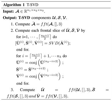
Theorem 1 (T-SVD) Suppose that L is an arbitrary invertible linear transform and
. Then, T-SVD of
is given by
(10)
where
,
, and
is an F-diagonal tensor.
The specific process will be presented in algorithm 1
Definition 7 (Tensor multi-rank and tubal rank) For
, let L be an arbitrary invertible linear transform satisfying
with
being a constant. The tensor multi-rank is a vector denoted as
. The tensor tubal rank is defined as the number of nonzero singular tubes of
, i.e.,
(11)
Definition 8 (TNN) Assume that
with corresponding T-SVD
; its tensor nuclear norm is defined as the sum of the singular values of all frontal slices of
, i.e.
(12)
Theorem 2 (Tensor Singular Value Thresholding) For any
and
, the solution of the problem
(13)
is given by
, which is defined as
(14)
where
with
.
Definition 9 (Tensor Frobenius norm (TFN)) For any
, the tensor Frobenius norm of
is defined as
(15)
2.3. Background
In this section, we briefly review the early work related to RPCA, and then discuss some recent developments of TRPCA and its application in computer vision.
RPCA tries to separate a low rank matrix
and a sparse matrix
from their sum
. As shown in [2], when the underlying tensor
satisfies the matrix incoherence conditions, the solution of the following problem:
(16)
can highly recover
and
with high probability with parameter
. In order to solve (16), various methods have been proposed [27]. Among them, Alternating Direction Method of Multipliers (ADMM, or also known as inexact augmented Lagrange multiplier) are widely used. In addition, Zhou et al. and Agarwal et al. [1] proved that even under small noise measurements, convex approximation by nuclear norm can still achieve bounded and stable results.
Unlike the matrix case, it is very difficult to define tensor rank. Many versions of tensor rank are proposed [5] [28]. Using the matricization, converting the tensor into matrix, Lu et al. [14] introduced the tensor nuclear norm as
, where
. Then, TRPCA is then given by
But the rank function may not be well approximated by nuclear norm. To overcome this problem, the T-TNN method was proposed in [29], which proposes a new definition of tensor nuclear norm, extends the truncated nuclear norm from the matrix case to the tensor case:
Afterwards, Jiang et al. [2] propose the partial sum of the tubal nuclear norm (PSTNN) of a tensor.
The tensor RPCA model using PSTNN was formulated as
The PSTNN is a surrogate of the tensor tubal multi-rank. Though PSTNN is a better approximation to the rank function, the stability issue is still challenging.
3. Tensor Robust Principal Component Analysis Based on Mixed Truncated Norm (T-HTN)
In this section, we mainly introduce the tensor truncated nuclear norm(T-TNN) and tensor truncated Frobenius norm (T-TFN) newly defined in this paper, and propose a tensor hybrid truncated norm(T-HTN) regularization model to improve effectiveness and stability. In addition, the iterative strategy is given.
3.1. T-HTN Model
As mentioned earlier, T-TNN is a better approximation of the rank function, which only considers the last min
singular value [30]. Since Frobenius norm can improve stability, we consider using Frobenius norm term to enhance stability, but the traditional Frobenius norm still needs to consider all singular values, which will make our T-TNN ineffective, which urges us to only consider the last min
singular values for enhancing stability in the definition of Frobenius norm. Based on these analyses, we will construct a more reasonable regularization term called “tensor truncated Frobenius norm (T-TFN)” to replace the original Frobenius norm and match it with T-TNN. Firstly, we give the T-TNN and T-TFN defined in this paper:
Definition 10 (Tensor truncated nuclear norm (T-TNN)) For
, the tensor truncated nuclear norm
is defined as the sum of the last min
singular values of all frontal slices of
, i.e.,
(17)
where
denotes the j-th largest singular value of
.
Definition 11 (Tensor truncated Frobenius norm (T-TFN)) Given a tensor
, the tensor truncated Frobenius norm (T-TFN) nuclear norm
is defined as the square root of the square sum of the last min
singular values of all frontal slices of
, i.e.,
(18)
Therefore,
can be defined as
(19)
Evidently, T-TFN could perfectly correspond to T-TNN as they both only concern the influence of the last min
singular values. Therefore, the two can be combined to establish a more effective hybrid truncated tensor robust principal component model (T-HTN):
(20)
Since
is nonconvex, it is not easy to solve the model (19). To this end, we establish the following theorems.
Theorem 3 For any
with corresponding T-SVD
, the following formula holds:
(21)
Theorem 4 For any
with corresponding T-SVD
, the following formula holds:
(22)
Through the above theorems, Equation (19) can be rewritten as
(23)
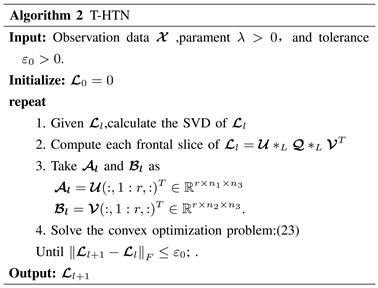
3.2. Solving Scheme
In order to solve the optimization problem (22), we will exploit an efficient iterative approach, which is divided into two steps. Firstly, we define
as the initial value of
. At the l-th iteration, fix
and perform the T-SVD with
, where
,
,
, we set
,
. Then fixing
and
, we can update
and
by solving the next convex optimization problem:
(24)
In short, we implement these two steps and alternate between them until the iterative scheme meets the tolerance error. Algorithm 2 outlines the complete procedure for (22). Now the remaining key issue is how to solve the model (23), which will be discussed in the next subsection.
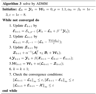
3.3. Optimization
In this section, an efficient iterative optimization scheme is created to optimize (23). According to the augmented Lagrangian multiplier method, the commonly used strategy is to approximately minimize the augmented Lagrangian function by adopting an alternating scheme, which we use to solve the model (23). To make the variables separable, we introduce the auxiliary variable
, thus (23) is equivalent to the following form:
(25)
The augmented Lagrange function of (24) can be written as:
(26)
where
is the Lagrange multiplier matrix and
is the penalty parameter. So, we can adopt the alternating iteration strategy, i.e., fix some variables and solve the remaining one.
Step 1: Keep
unchanged and update
through
(27)
Step 2: Keep
unchanged and update
through
(28)
Obviously, Equation (27) is a quadratic function about
. Let
be a function with respect to
, then
can be approximated by the linearization at
:
where
is a parameter, and
denotes the gradient of the function
at
. Thus, (27) with respect to
can be reformulated as:
(29)
By Theorem 1 and Theorem 2, this could be solved as
(30)
Step 3: Keep
unchanged and update
through
(31)
Obviously, the objective function of (30) is a quadratic function. Through a simple derivation operation, we get
This means that
(32)
Step 4: Update Lagrange multipliers
,
:
(33)
To sum up, algorithm 3 gives a complete program.
3.4. Adaptive Parameter
Previous studies have shown that the computational cost could increase significantly, since the algorithm may converge slowly when the fixed penalty parameter
and
are chosen too small or large [28] [29], and we need to constantly try different values to pick a good value of
and
. It is not easy to choose the optimal
and
. Accordingly, a dynamical
and
may be required to accelerate convergence in real applications. With the aid of the way in [31], the following adaptive update criterion is used:
(34)
(35)
where
and
is an upper bound of
and
, and
is defined as:
(36)
(37)
where
and
are constant and
is a threshold chosen in advance.
3.5. Convergence Analysis
This section discusses the convergence of the proposed algorithm.
Firstly, the optimal value of Equation (24) is expressed as follows
(38)
The augmented Lagrange function is written as
(39)
In addition, in order to further analyze the convergence of the algorithm, the following three lemmas are established
Lemma 2 Let
be the optimal solution of the augmented Lagrange function (38) and satisfy
, then:
(40)
where
is the solution of the
-th iteration in the algorithm 3,
is the k-th iterative solution of (38).
.
Lemma 3 Let
,
,
,
then the following inequality holds:
(41)
Lemma 4 Let
be the optimal solution of the augmented Lagrange function (38) and
,
, define:
(42)
Then
is decreasing in each iteration and satisfies the following relationship:
(43)
According to the above results, the following convergence theorems are obtained:
Theorem 5 Based on the conditions in lemmas 2, 3 and 4, the iterative solution
, when
.
4. Experiments
In this section, we will conduct numerical experiments to confirm our main results. We studied the ability of T-HTN to recover various tube rank tensors from various sparse noises, and applied T-HTN to image denoising.
4.1. Synthetic Data Experiments
In this section, we compare the accuracy and speed of T-HTN and TNN based TRPCA [22] on synthetic datasets. Given tensor size
and tubal rank
, we first generate a tensor
by
,where the elements of tensors
,
are sampling from independent identically distributed (i.e.) standard Gaussian distribution. Then, we from
by
. Next, the support of
is uniformly sampled at random. For any
, we get
, where
is a tensor with independent Bernoulli ±1 entries. Thus, we get the observation tensor
. In the experiment part, we set the parameters
. We use the relative square error (RSE) to evaluate the estimated
of the underlying tensor
, that is
.
4.1.1. Effectiveness and Efficiency of T-HTN
Firstly, we prove that T-HTN can accurately recover the underlying tensor
. Based on experience, we test the recovery performance of tensors of different sizes by setting
and
, with
. Then a more difficult setting
is tested. The results are shown in Table 1. and
Table 2. It is not difficult to see that T-HTN and TRPCA have the same good recovery performance, because both can accurately recover the underlying tensor, but T-HTN has obvious advantages in time.
To test the influence of the distribution of outliers on T-HTN performance, we obtain the outlier tensor element
from i.i.d Gaussian distribution
, or uniform distribution
. The corresponding results are given in Table 3 and Table 4. The performance of T-HTN and TRPCA is not significantly affected by the outlier’s distribution. This phenomenon can be explained by Theorem 4.1 in [22], that is when the outlier tensor
is uniformly distributed, TRPCA can accurately restore the underlying tensor
under some mild conditions. In [22], only one hypothesis is made for the random location distribution, but no hypothesis is made for the size or symbol of non-zero terms. Because the T-HTN proposed in this paper can well simulate TRPCA with low tube rank tensors, T-HTN is also robust to outlier.
![]()
Table 1. Comparison with TRPCA [22] in both accuracy and speed for different tensor sizes when
.
![]()
Table 2. Comparison with TRPCA [22] in both accuracy and speed for different tensor sizes when
.
![]()
Table 3. Comparison with TRPCA [22] in both accuracy and speed for different tensor sizes when the outlier tensor element
from i.i.d Gaussian distribution
.
![]()
Table 4. Comparison with TRPCA [22] in both accuracy and speed for different tensor sizes when the outlier tensor element
from i.i.d Gaussian distribution
.
In order to further verify the efficiency of the proposed T-HTN, we consider a special case: fixing the tubal rank of the underlying tensor
and changing the size of the underlying tensor
. Explicitly, we fix
, and vary
with
. We tested each data 10 times and calculated the average time. Figure 1 shows the relationship between average time and tensor size. Obviously, both can accurately recover the underlying tensor, but in terms of running time, TRPCA expands super-linearly and T-HTN expands approximately linear scaling.
4.1.2. Effects of the Number of Truncated Singular Values
The performance of T-HTN largely depends on the number of truncated elements of
in (23), that is, the number of singular values to be retained. Here, we discuss the influence of different truncation degrees of Frobenius norm and nuclear norm on the accuracy and speed of T-HTN. Specifically, we consider the tensor with the size of
and set up four different truncation methods
and sparsity
as
, where the elements outliers follow i.i.d.
. By varying the initialized
. Firstly, we give the effect of the number of truncated singular values on the recovery performance of the underlying tensor
.The results are shown in Figure 2. There is a phrase transition point
. Once the reserved singular valuer is greater than it, the RSE of
will decrease rapidly. Then, we give the influence of the number of truncated singular values on the estimation performance of outlier tensor
. Figure 3 shows the RSE and
-norm of
finally solved. Finally, we show the effect of the number of truncated singular values on the running time of T-HTN in Figure 4. Obviously, the more singular values remain, the longer the running time, and the more complex the underling tensor becomes, which is also consistent with our intuition.
4.2. Real Data Experiments
In this section, we evaluate the efficiency of T-HTN proposed in this paper on real data sets and compare it with TRPCA. Specifically, we do tensor restoration experiments on color image data. The purpose is to restore the original image from its corrupted observation. For the estimation
of the underlying tensor
, we choose the relative square error(RSE), the peak signal-to-noise ratio (PSNR), and the structured similarity index(SSIM) as the evaluation index, which is respectively defined as,
![]()
Figure 1. Computation time of TRPCA and proposed T-HTN.
![]()
Figure 2. Effects of initialized tubal rank r on the recovery performance of the underlying tensor L.
![]()
Figure 3. Effects of initialized tubal rank r on the recovery performance of the underlying tensor E.
![]()
Figure 4. Effects of initialized tubal rank r on the running time of T-HTN.
and
where
and
are the average values of original tensor and recovered tensor represents the covariance of
and
,
and
respectively denotes the standard deviation of
and
. Natural scenes images follow natural statistics [32]. As shown by Hu et al. [33], information of image scenes is dominated by the top 20 singular values, which is low-rank. In Figure 5, our experimental data are from 10 common color images. The size of the selected images is
. When these color images are converted into matrices, they can be regarded as low rank structures. The same is true for tensor data.
![]()
Table 5. PSNR values of different truncated singular values.
Number of Optimal Truncated Singular Values
First, we apply our algorithm to a picture data. We need to preset the number of truncated singular values. Therefore, we designed an experiment in this part, set the number of reserved singular values to
, test all possible values, and select the best value. We test 10 images and selected the number of optimal truncated singular values. The detailed results are shown in Table 5. In the worst case of our approach, it is sufficient to test
from 1 to 20. Even if the best
is not selected, its effectiveness will not be lost.
4.3. Conclusions
This paper introduces a new regularization term T-TFN, integrates T-TFN and T-TNN, and proposes a new model T-HTN for TRPCA. Because of the emergence of T-TFN, this new T-HTN regularization method can improve the effectiveness and stability of the model. Then, an effective iterative framework is designed to solve the new optimization model. In addition, its convergence is also derived in the mathematical field. The experimental results on synthetic data, real visual images and recommendation systems, especially the use of statistical analysis methods, illustrate the advantages of HTN over other methods. In other words, HTN method is more effective and stable.
There is still room for further research in this field, for example, how to prove the stability of the proposed method mathematically, and how to select the proportion of missing elements to ensure some theoretical analysis of effective performance.
This work is supported by Innovative talents support plan of colleges and universities in Liaoning Province (2021).