Cox Proportional Hazard Model for Survival Time of Neonatal Mortality in Neonatal Intensive Care Unit of Hospitals in River Nile State-Sudan

Abdellateef Khalifa Hamid Ali^1*, Amin Ibrahim Adam Mohammed²

¹Faculty of Mathematical Science, El-Fashir University, El-Fashir, Sudan.
²Faculty of Economics & Political Sciences, Omdurman Islamic University, Omdurman, Sudan.

DOI: 10.4236/ojs.2022.125038                

Abstract

Cox Proportional Hazard model is a popular statistical technique for exploring the relationship between the survival time of neonates and several explanatory variables. It provides an estimate of the study variables’ effect on survival after adjustment for other explanatory variables, and allows us to estimate the hazard (or risk) of death of newborn in NICU of hospitals in River Nile State-Sudan for the period (2018-2020). Study Data represented (neonate gender, mode of delivery, birth type, neonate weight, resident type, gestational age, and survival time). Kaplan-Meier method is used to estimate survival and hazard function for survival times of newborns that have not completed their first month. Of 700 neonates in the study area, 25% of them died during 2018-2020. Variables of interest that had a significant effect on neonatal death by Cox Proportional Hazard Model analysis were neonate weight, resident type, and gestational age. In Cox Proportional Hazard Model analysis all the variables of interest had an effect on neonatal death, but the variables with a significant effect included, weight of neonate, resident type and gestational age.

Keywords

Neonatal Mortality, Cox Proportional Hazard Model, Survival Function, Haz-ard Function, Kaplan-Meier Method

1. Introduction

Survival data is a term used for describing data that measure the time of a certain event. In survival analysis, the event may be death, the occurrence of disease (or complication), time to an epileptic seizure, time it takes for a patient to respond to therapy, or time from response until disease relapse (i.e., disease returns). In demography, the event can be entering marriage.

The event is a transition from one state to another. Death is a transition from state alive to state dead. Time to an event is a positive real-valued variable having continuous distribution. It is necessary to define the starting time point, say 0, from which times are measured. When we measure age, the starting time point may be the date of birth. In biomedical applications, the data are collected over a finite period of time and consequently the “time to event” may not be observed for all the individuals in our study sample [1].

If the endpoint is the death of a patient, the resulting data are literally survival times. However, data of a similar form can be obtained when the end-point is not fatal, such as the relief of pain, or the recurrence of symptoms. In this case, the observations are often referred to as time-to-event data [1].

Data are censored when we do not know their precise value, but only have some bounds on them. An observation t is left-censored if we only know that t < c for some c, it is right-censored if we only know that t > c and it is interval-censored if what we know is that a < t < b for some numbers a and b. Censored observations occur also for data that are not time-to-event data [2].

In essence, censoring occurs when we have some information about individual survival time, but we don’t know the survival time exactly. Left censoring occurs when the event proceeded during the observation period. Right censoring arises when the event either never occurred or took place after the period of observation, and can come about due to a loss-to-follow-up, refusal to participate after initial enrollment, or the end of the observation period. In a study of mortality, however, death constitutes the event, not a reason for censoring. In survival analysis the measure of effect typically obtained is called a hazard ratio [3].

The neonatal period (from birth to the 28^th day of life) is normally considered to be the most vulnerable and high-risk time in neonate life because of the highest mortality and morbidity incidence in human life during that period. During this period the neonate risk of death is almost 15 times more than at any other time before the first birthday [4].

Criteria for admission to the normal newborn nursery or couplet care with the mother vary among hospitals. The minimum requirement typically is a well-appearing infant of at least 35 weeks gestational age, although some nurseries may specify a minimum birth weight, for example, 2 kg [5].

Many communities have adapted to this situation by not recognizing the birth as complete, and by not naming the child until the newborn infant has survived the initial period. Health workers at primary and secondary levels of care often lack the skills to meet the needs of newborn infants, since the recognition of opportunity is only just emerging in countries, and their experience in this area is therefore limited. Each neonatal death can be further clarified into viable and non-viable deaths depending on the gestational age at which they were born, and where they were born [4].

The data used for this paper is secondary data from medical statistics & records at hospitals of study areas which consist of nurseries in it. I was chosen as sample size 700 medical records of newborns admitted to nurseries of those hospitals. And then get the data according to the variables of interest.

This paper is organized as follows: Introduction, Materials and methods (theoretical aspect, practical aspect, analysis and results), Discussion and Conclusion.

This paper is related to some papers, one of them in title used Cox PH model for Age at First Sexual Intercourse in Nigeria & other in title ITN-Factor Impact on Mortality Due to Malaria. The important results of these papers are as the following: The median age of first sexual intercourse is 16 years which implies that about 50% of the respondents had their first sexual intercourse on or before their 16th birthday. Education, religion, region and residence significantly affect the age of first sexual intercourse while circumcision has no significant effect.

Sex of patient was insignificant to deaths due to malaria. Age of patient and user status was both significant. The magnitude of the coefficient (0.384) of ITN user status depicts its high contribution to the variation in the dependent variable.

2. Materials and Methods

2.1. Theoretical Aspect

The survivor function S(t) gives the probability that a person survives longer than some specified time t that is, S(t) gives the probability that the random variable T-exceeds the specified time t. The survivor function is fundamental to a survival analysis, because obtaining survival probabilities for different values of t provides crucial summary information from-survival data. In practice, when using actual data, we usually obtain graphs that are step functions, as illustrated here, rather than smooth curves. Moreover, because the study period is never infinite in length and there may be competing risks for failure, it is possible that not everyone studied gets the event. The estimated survivor function, denoted by a caret over the S in the graph, thus may not go all the way down to zero at the end of the study [6].

The basic quantity employed to describe time-to-event phenomenon is the Survival Function S(t), and it is defined as:

$S\left(t\right)=P\left(T>t\right)=1-P\left(T\le t\right)$ (2.1)

the probability of an individual survives beyond time t.

Since a unit either fails, or survives, and one of these two mutually exclusive alternatives must occur, we have:

$S\left(t\right)=1-F\left(t\right)$, $F\left(t\right)=1-S\left(t\right)$ (2.2)

where F(t) is the cumulative distribution function (CDF). If T is a continuous random variable, then S(t) is a continuous, strictly decreasing function. The survival function is the integral of the probability density function (pdf), f(t), that is:

$S\left(t\right)={\displaystyle \underset{t}{\overset{\infty }{\int }}f\left(x\right)\text{d}x}$ (2.3)

Thus,

$f\left(t\right)=-\frac{\text{d}S\left(t\right)}{\text{d}t}$

The probability distribution of survival times can be characterized by three functions, one of which is known as the hazard function. Given a set of data, the users of statistics would like to calculate the mean and standard deviation. Investigators have learned that the problem with survival time data is that the mean survival time depends on when the data is analyzed. The unique feature of survival data is that the subjects typically join the study at different time points, may withdraw from the study, or may be lost to follow-up. Thus, the value of the average survival time will change as time elapses until the point at which the lifetimes of all of the implants in the study have been observed. In survival analysis, it is often unrealistic to expect a set of data without any censored observations [7].

The procedure, called the hazard function, is defined as the probability that an implant fails in a time interval between t and t + ∆t, given that the implant has survived until time t. In statistics, this concept is known as the conditional probability. In engineering, the term instantaneous failure rate and in epidemiology, the term force of mortality is more commonly used. The hazard function is a measure of the likelihood of failure as a function of the age of the individual implants. The hazard function reflects the risk of failure per unit time during the aging process of the implant. It plays an important role in the study of survival times [7].

The next instant the failure rate may change and the individuals that have already failed will play no further role since only the survivor’s count. The failure rate (or hazard rate) is denoted by h(t) and is defined by the following equation:

$h\left(t\right)=\underset{h\to 0}{\lim }\frac{P\left(t\le T\le t+h/T\ge t\right)}{h}$ (2.4)

The failure rate is sometimes called a “conditional failure rate” since the denominator S(t) (i.e., the population survivors) converts the expression into a conditional rate, given survival past time t. From Equation (2.4), by the theorem of conditional probability and omitting suffix T, we get expression of hazard function as:

$h\left(t\right)=\frac{f\left(t\right)}{S\left(t\right)}=\text{instantaneous}\left(\text{conditionalfailurerate}\right)$ (2.5)

So, hazard at time t is potential per unit time for the event to occur given that the subject has survived till t. basically, it the rate of event at time t.

It is clear from the expression and definition that hazard is a rate rather than being a probability. Its value ranges from zero to infinity [1].

The Kaplan-Meier curve is a nonparametric estimate of the survival curve, and it is an estimator based on the products of conditional probabilities, it is also sometimes called the product-limit estimator. The Kaplan-Meier curve starts out with S(t) = 1 for all t less than the first event time (such as a death at t₁) [8].

The tools that will be used in this paper are depicted in Diagram 1.

We introduce the product-limit (PL) method of estimating survival rates, also called the Kaplan-Meier method. Let t₁ < t₂ < … < t_k, be the distinct observed death times in a sample of size n from a homogeneous population with survival function S(t) to be estimated (k ≤ n; k could be less than n because some subjects may be censored and some subjects may have events at the same time). Let n_i be the number of subjects at risk at a time just prior to t_i(1 ≤ i ≤ k; these are cases whose duration time is at least t_i), and d_i the number of deaths at t_i. The survival function S(t) is estimated by

${\hat{S}}_{\left(t\right)}={\displaystyle {\prod }_{t_i\le t}\left(1-\frac{d_i}{n_i}\right)}$ (2.6)

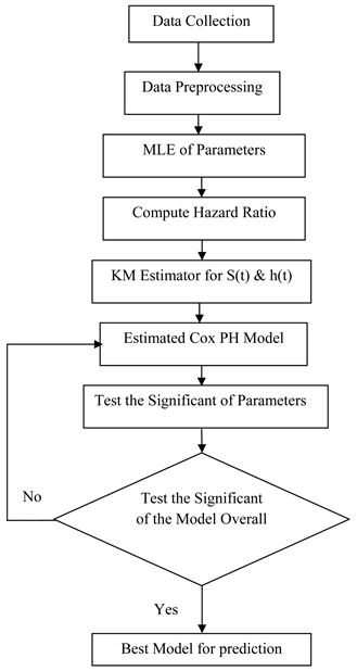
Diagram 1. The methodology flow diagram.

This is called the product-limit estimator or Kaplan-Meier estimator with a 95% confidence given by

${\hat{S}}_{\left(t\right)}\exp \left[\pm 1.96{\hat{s}}_{\left(t\right)}\right]$ (2.7)

The explanation could be simple, as follows: $d_i/n_i$ is the proportion (or estimated probability of having an event in the interval from $t_{i-1}$ to $t_i$, and $1-d_i/n_i$ represents the proportion (or estimated probability of surviving that same interval), and the product in the formula for ${\hat{S}}_{\left(t\right)}$ follows from the product rule for probabilities [9].

A natural way of estimating hazard function for unground survival data is to take the ratio of the number of deaths at a given death time to the number of individuals at risk at that time. If the hazard function is assumed to be constant between successive death times, the hazard per unit time can be found by further dividing by the time interval [3].

Thus if there are d_j deaths at j^th death time $t_{\left(j\right)}$ $j=1,2,\cdots ,T$, and $n_j$ at risk at time $t_{\left(j\right)}$, the hazard function in the interval from $t_{\left(j\right)}$ to $t_{\left(j+1\right)}$ can be estimated by Kaplan-Meier estimator as follows:

${\hat{h}}_{\left(t\right)}=\frac{d_j}{n_j{T}_j}$ (2.8)

We note that since ${\hat{h}}_{\left(t\right)}$, $t_{\left(j\right)}\le t<t_{\left(j+1\right)}$, is an estimate of the risk of death per unit time in the j^th interval, the probability of death in that interval is ${\hat{h}}_{\left(t\right)}{T}_j$ that is $d_j/n_j$. Hence an estimate of the corresponding survival probability in that interval is $1-\left(d_j/n_j\right)$ [3].

There are two broad reasons for modeling survival data. One objective of the modeling process is to determine which combinations of potential explanatory variables affect the form of the hazard-function. In particular, the effect that the treatment has on the hazard of death can be studied, as can the extent to which other explanatory variables affect the hazard function. Another reason for modeling the hazard function is to obtain an estimate of the hazard function itself for an individual [10].

The basic model for survival data to be considered in this paper is the proportional hazards model. This model was proposed by Cox (1972) and has also come to be known as the Cox regression model. Although the model is based on the assumption of proportional hazards, no particular form of probability distribution is assumed for the survival times. The model is therefore referred to as a semi-parametric model [10].

The purpose of the model is to evaluate simultaneously the effect of several factors on survival. In other words, it allows us to examine how specified factors influence the rate of a particular event happening at a particular point in time [11].

The cox proportional hazards model can be generalized to the situation where the hazard of death at a particular time depends on the values $x_1,x_2,\cdots ,x_p$ of p explanatory variables. The values of these variables will be assumed to have been recorded at the time origin of the study.

An extension of the model is to cover the situation where the values of one or more of the explanatory variables change over time. The set of values of the explanatory variables in the proportional hazards model will be represented by the vector $X$, so that $X=x_1,x_2,\cdots ,x_p$ . Let $h_0\left(t\right)$ be the hazard function for an individual for whom the values of all the explanatory variables that make up the vector x are zero [10].

For a categorical explanatory variable, a reference level (usually the first or last level of the variable) will be chosen and the other levels of the explanatory variable will be compared with the chosen reference level. The Cox model assumes that the hazard ratio of any two individuals is constant over time [12].

Under the proportional hazards models, the hazard h(t) is modeled as:

$h\left(t,x\right)=h_0\left(t\right)\exp \left({\beta }_1{x}_1+{\beta }_2{x}_2+\cdots +{\beta }_k{x}_k\right)$ (2.9)

where $x_1,x_2,\cdots ,x_k$ are a collection of independent variables, and $h_0\left(t\right)$ is baseline hazard at time t, rerenting the hazard for a person with the value 0 for all the independent variables, ${\beta }_k$ are the coefficients of the parameters and t survival time. The hypothesis $H_1\#{\beta }_k=1$ versus $H_1\#{\beta }_k\ne 1$ can be tested as follows:

• Compute the test statistics $Z={\hat{\beta }}_k/se\left({\hat{\beta }}_k\right)$.

• To conduct a two sided level α significant test, if $Z<Z_{\alpha /2}$ or $Z>Z_{1-\alpha /2}$ [13].

Consider an observed sample $y=\left(y_1,\cdots ,y_n\right)$ and likelihood function $L\left(\beta \right)=L\left(\beta ;y\right)$ Recall that the likelihood associated with a particular parameter value ${\beta }_0$ is the probability (density) of obtaining the sample y, assuming that the true value of the parameter is ${\beta }_0$. This measures the support that the data has for the parameter value ${\beta }_0$, and the most supported parameter value $\hat{\beta }$ will be the value for which $L\left(\hat{\beta }\right)>L\left({\beta }_0\right)$ whenever ${\beta }_0=\hat{\beta }$.

The most supported parameter value is therefore the value that achieves the highest likelihood possible based on the likelihood function $L\left(\beta \right)$, or in other words maximizes the likelihood function. Since this value has more support from the data than any other parameter value it makes sense to use it as our estimate. This approach to estimation is referred to as maximum likelihood estimation and can be interpreted as providing the parameter value that makes the observed sample the most likely sample among all possible samples. The estimate that arises from using this approach, which will be a function of the observed sample $\hat{\beta }=\varnothing \left(y\right)$, is referred to as the maximum likelihood estimate. As with any estimate, it is the observed value of a random variable, the maximum likelihood estimator $\hat{\beta }=\varnothing \left(y\right)$. The abbreviation MLE is used interchangeably to refer to either the maximum likelihood estimates or the maximum likelihood estimator, depending on the context [14].

Maximum likelihood estimation provides a general approach to estimating a parameter, and can in principle be applied in any situation where we have a likelihood function. Bearing in mind these potential complexities, an MLE is strictly speaking defined as any value $\hat{\beta }$ that is in the parameter space and for which $L\left(\hat{\beta }\right)>L\left({\beta }_0\right)$ for any other parameter value ${\beta }_0$ that is also in the parameter space. In mathematical parlance, we say that the MLE is the value that maximizes $L\left(\beta \right)$ over the parameter space. In practice, however, this often simply amounts to taking the MLE to be the single value of θ that leads to function $L\left(\beta \right)$ taking on its highest possible value [14].

As a final point of importance in defining the MLE, if a particular parameter value maximizes the likelihood function, then it will also maximize the log-likelihood function. Thus, the above definition of the MLE can also be made with respect to the log-likelihood $\log L\left(\beta \right)$ rather than the likelihood $L\left(\beta \right)$. In practice, this fact is often used for computation purposes because the log-likelihood function is usually a more mathematically convenient function to deal with [14].

This is generally done by maximizing the natural log of L, which is computationally easier. The maximization process is carried out by taking partial derivatives of log of L with respect to each parameter in the model, and then solving a system of equations. Then the Cox PH model formula after estimation can be written as follows:

$\hat{h}\left(t\right)={\hat{h}}_0\left(t\right)\exp \left({\hat{\beta }}_1{x}_1+{\hat{\beta }}_2{x}_2+\cdots +{\hat{\beta }}_P{x}_P\right)$ (2.10)

Once the ML estimates are obtained, we are usually interested in carrying out statistical inferences about hazard ratios defined in terms of these estimates. The estimated hazard ratio (HR) was computed by exponentiation the coefficient of a (0, 1) exposure variable of interest. Note that the model contained no interaction terms involving exposure [6].

The quantities $\exp \left({\beta }_i\right)$ are called Hazard Ratios (HR), if HR = 1 there is no effect, if HR < 1 there is an effect with decrease in the risk or the hazard and if HR > 1 there is an effect by increase in the hazard. The Cox model assumes that the hazard ratio of any two individuals is constant over time. For a categorical explanatory variable, a reference level (usually the first or last level of the variable) will be chosen and the other levels of the explanatory variable will be compared with the chosen reference level [6].

2.2. Practical Aspect

2.2.1. Data Description

The data used for this study is a secondary data from the 2018-2020 NICU in Hospitals of River Nile State of 700 respondents (Newborns). Six explanatory variables were considered to study their effect on survival time of newborn. The censoring nature of the data made us to use Cox Proportional Hazard Model to analyses the effects of factors on survival time of neonate. Some of the respondents in the study were censored since they did not have the event of interest (newborn death).

2.2.2. Analysis and Results

From applied of descriptive statistics & Kaplan-Meier method of survival and Hazard function, and construction Cox Proportional Hazard model to assess the variable of interest related to newborn data. We found that:

From Table 1 we noticed that the mean of weight of newborn is 2.4 kg, minimum value of it is 0.36 kg, and maximum value is 6 kg. The mean of gestational age is 33 weeks, minimum value of it is 22 week, and maximum value is 47 week. The mean of survival time of newborns is 4 days, minimum value of it is one day, and maximum value is 29 days.

From Table 2 and Figure 1 we noticed that 25% of newborns from sample of study area is dead, this percentage can be considered as a high percentage of neonatal mortality in study area, which newborns of it can be exposure to the risk of death with that percentage.

From Table 3 & Table 4 and Figure 2 we notice that the KM curve for group 2 is consistently higher than the KM curve for group 1. These figures indicate

Figure 1. Case processing summary for the study sample of newborn’s data. source: Prepared by the researcher using Excel.

Table 1. The mean, minimum and maximum for the variables, weight of newborn by kg, Gestational age by weeks and Survival Time by days.

Source: Prepared by the researcher using SPSS.

Table 2. Case processing summary for the study sample of newborn’s data.

Source: Prepared by the researcher using SPSS.

Table 3. Survival function for male.

Source: Prepared by the researcher using SPSS.

Table 4. Survival function for female.

Source: Prepared by the researcher using SPSS.

that group 2, which is the female group, has better survival prognosis than group 1, the male group. However, the KM curves are very close during the first five days, but are quite separate after five days, although they appear to come close again around seventeen days. The males of newborns were more exposure to the risk of death.

Figure 2. Kaplan-meier estimates of survival & hazard functions for gender of newborn. Source: Prepared by the researcher using SPSS.

From Table 5 & Table 6 and Figure 3 we found that group 1 (normal delivery) appears to have consistently better survival prognosis than group 2 (caesarian section delivery). However, the KM curves are very close from the first days until day twenty, but are quite separate after twenty days. The newborns which delivered with caesarian section were more exposure to the risk of death.

From Table 7 & Table 8 and Figure 4 we notice that the KM curve for group 2 (twin+) is consistently higher than KM curve for group 1 (singleton). These figures indicate that the twin+ group has so better survival prognosis than the singleton group. KM curves are very close from the first days until day fifteen. After ten days to twenty days the curve of two groups had a same probability of survival approximately. Singleton type of birth for newborns was more exposure to the risk of death.

Figure 3. Kaplan-meier estimates of survival & hazard functions for mode of delivery. Source: Prepared by the researcher using SPSS.

Table 5. Survival function for normal delivery.

Source: Prepared by the researcher using SPSS.

Table 6. Survival function for caesarian delivery.

Source: Prepared by the researcher using SPSS.

Table 7. Survival function for singleton newborn.

Source: Prepared by the researcher using SPSS.

Figure 4. Kaplan-meier estimates of survival & hazard functions for birth type. Source: Prepared by the researcher using SPSS.

Table 8. Survival function for twin+ newborn.

Source: Prepared by the researcher using SPSS.

From Tables 9-11 and Figure 5 we conclude that KM curves are quite different with group 3 (weight more than 4.35) having consistently better survival prognosis than group 2 (weight in period 2.35 - 4.35), as the group 3 (weight more than 4.35) had a few cases, we can just say the group 2 (weight in period 2.35 - 4.35) having consistently better survival prognosis than group 1 (weight in period 0.35 - 2.35). Note also the difference between group 1 and 2 is about the same over time until before 25 days, whereas group 2 appears to diverge from group 3 as time increases. we found about 36% of newborns with weight in period (0.35 - 2.35 kg) were exposure to the event of death, also 16% of newborns were exposure to the event of death when their weighs of in period (2.35 - 4.35 kg), and then the newborns which their weight are more than 4.35 kg, exposure to the event of death with 10%. That means the weight of newborn in period (0.35 - 2.35 kg) had a high risk of death.

Figure 5. Kaplan-meier estimates of survival & hazard functions for weight of newborn by kg. Source: Prepared by the researcher using SPSS.

Table 9. Survival function for weight of newborn in period (0.35 - 2.35 kg).

Source: Prepared by the researcher using SPSS.

Table 10. Survival function for weight of newborn in period (2.35 - 4.35 kg).

Source: Prepared by the researcher using SPSS.

Table 11. Survival function for weight of newborn more than 4.35 kg.

Source: Prepared by the researcher using SPSS.

From Table 12 & Table 13 and Figure 6 we notice that the KM curve for group 1 is consistently higher than KM curve for group 2. These figures indicate that the group 1, which is Urban Resident, has better survival prognosis than group 2 the Rural Resident. However, the KM curves are very close from the first days until day twenty, but are quite separate after twenty days. We found 30% of the newborns in Rural Resident were exposure to the event of death, and 19% of them in Urban Resident were exposure to the event of death in the study area. That let us to say newborns in Rural Resident had a high risk of death.

Table 12. Survival function for urban resident.

Source: Prepared by the researcher using SPSS.

Table 13. Survival function for urban resident.

Source: Prepared by the researcher using SPSS.

Figure 6. Kaplan-meier estimates of survival & hazard functions for resident type. Source: Prepared by the researcher using SPSS.

From Tables 14-16 and Figure 7 we notice that the KM curves for group 3 (gestational age more than 42 week) having consistently so better survival prognosis than the KM curve for group 2 (gestational age in period 32 - 42 week), as the group 3 (gestational age more than 42 week) had a few cases, we can just say the group 2 (gestational age in period 32 - 42 week) having consistently better survival prognosis than group 1 (gestational age in period 22 - 32 week). Note also that the difference between group 1 and 2 is about the same over time. we noticed about 48% of newborns were exposure to the risk of death when their gestational age in period (22 - 32 week), also 21% of newborns with gestational age in period (32 - 42 week), were exposure to the risk of death, and then the newborns which their gestational age more than 42 week had a very few cases, so they cannot be exosured to risk of death. This means that the gestational age with period (22 - 32 kg), had a high risk of death.

Table 14. Survival function for gestational age in period (22 - 32 week).

Source: Prepared by the researcher using SPSS.

Table 15. Survival function for gestational age in period (32 - 42 week).

Source: Prepared by the researcher using SPSS.

Table 16. Survival function for gestational age more than 42 week.

Source: Prepared by the researcher using SPSS.

Figure 7. Kaplan-meier estimates of survival & hazard functions for gestational age by weeks. Source: Prepared by the researcher using SPSS.

Table 17 explain that the result of Maximum Likelihood Ratio Test to test the significant of the model overall, when the sig (p-value) for the test statistics is 0.00 which less than 0.05 then that was evidence of significant of the estimated model.

From Table 18 we found that:

There is no significant difference for the risk of death on the Gender of newborn, because Wald test value is 1.80 with p-value 0.180 which it is greater than 0.05, there is no significant difference in Mode of Delivery to the risk of death for newborn, because Wald test value is 0.015 with p-value 0.902 which it is greater than 0.05, and there is no significant difference on Birth Type to the risk of death for newborn, because Wald test value is 0.046 with p-value 0.830 which it is greater than 0.05.

There is a significant effect Weight of newborn on the event of death for newborn, when the Wald test 9.464 with p-value 0.002 which it is less than 0.05,

Table 17. Tests of model coefficients.

Source: Prepared by the researcher using SPSS.

Table 18. Cox proportional hazard model on risk factors of neonatal mortality.

Source: Prepared by the researcher using SPSS.

the hazard of event of death for newborns which their weight in period (0.35 - 2.35 kg), decrease by [(1 − 0.607) × 100] 39.3% respectively when compared with weight of newborn in periods (2.35 - 4.35 kg & more than 4.35 kg). As weight of newborn decreases, the hazard of event of death increased (1 ÷ 0.607) = 1.6 times, respectively that of weight of newborn in period (0.35 - 2.35 kg). That means the weight of newborn in period (0.35 - 2.35 kg), is more exposure to the risk of death than other weights of newborn periods (2.35 - 4.35 kg & more than 4.35 kg).

There is a significant effect of Resident type on newborn death, according to Wald test value 8.946 with p-value 0.003 which it is less than 0.05, the hazard of event of death for newborns which living at Urban Resident decrease by [(1 − 0.629) × 100] 37.1% respectively when compared with Rural Resident. As the Resident Type changes, the risk of death for newborn increased (1 ÷ 0.629) = 1.5 times, respectively that of Rural Resident.

There is a high significant effect of Gestational Age on newborn death, according to p-value 0.000 is less than 0.05, the hazard of event of death for newborns with Gestational Age in period (22 - 32 week), decrease by [(1 − 0.629) × 100] 37.1% respectively when compared with Gestational Age periods (22 - 32 week & more than 42 week). As Gestational Age- decreases, the hazard of event of death for newborns increased (1 ÷ 0.485) = 2.06 times or twice, respectively that of Gestational Age in period (22 - 32 week & more than 42 week).

Estimated Model for Cox Proportional Hazard for the survival time of neonatal mortality can be written as follows:

${\hat{h}}_{\left(t,X\right)}={\hat{h}}_{0\left(t\right)}\exp \left(0.22x_1+0.02x_2+0.06x_3-0.50x_4-0.46x_5-0.72x_6\right)$ (2.11)

when x₁ represent (gender of newborn take 1 = male, 2 = female), x₂ represent (mode of delivery take 1 = normal delivery, 2 = caesarian), x₃ represent (birth type 1 = singleton, 2 = twin+), x₄ represent (weight of newborn by kg take 1 = weight in period (0.35 - 2.35), 2 = weight in period (2.35 - 4.35), 3 = weight more than 4.35), x₅ represent (resident type 1 = urban, 2 = rural), x₆ represent (gestational age by weeks take 1 = gestational age in period (22 - 32), 2 = gestational age in period (32 - 42), 3 = gestational age more than 42).

As an example let $x_1=1$, $x_2=2$, $x_3=2$, $x_4=3.8\text{kg}$, $x_5=2$, $x_6=36$ week.

Substitute these values in Equation (2.11)

${\hat{h}}_{\left(t,X\right)}={\hat{h}}_{0\left(t\right)}\exp \left(0.22\left(1\right)+0.02\left(2\right)+0.06\left(2\right)-0.50\left(3.8\right)-0.46\left(2\right)-0.72(\; 36\; )\right)$

${\hat{h}}_{\left(t,X\right)}={\hat{h}}_{0\left(t\right)}\exp \left(-28.36\right)={\hat{h}}_{0\left(t\right)}4.8$

The baseline ${\hat{h}}_{0\left(t\right)}$ can be neglect, so

${\hat{h}}_{\left(t,X\right)}=4.8$

This means the risk of death for newborn with the above values of variable of interest will be 4.8.

3. Discussion

The variables of interest concerning health variables and social variables representing as gender of newborn (male, female), birth type (Single, Twin+), weight of newborn periods by kg (0.35 - 2.35, 2.35 - 4.35 and more than 4.35), mode of delivery (Normal, Caesarian), gestational age period by weeks (22 - 32, 32 - 42 and more than 42), and resident type (Urban, Rural). Various variables have been distinguished to be connected with neonatal mortality. Neonatal mortality studies can help the health sector to improve the maternal and newborns care, and then according to neonatal mortality rates in countries we can judge on that country which had a high neonatal mortality rates by developing country and the opposite is true.

This paper explain that the newborns which their weight period listed as (0.35 - 2.35) were more exposure to death than other periods (2.35 - 4.35 and more than 4.35), this result is reliable with a study entitle Using the Logistic Regression Model and Cox Regression to Study the Factors Affecting the Mortality of Infants in Palestine led in 2015, which concluded that the mother’s access to iron tablets during pregnancy and the results indicated that the mother’s access to health care during pregnancy and the low birth weight have a significant impact on the life of the infant.

In our paper, we expound that the risk of death for neonates who live in rural area is 1.5 times neonates that live urban area; this result can be found with a study led in Addis Ababa in 2013, which explain that the Contextual factors included in the analysis were urban-rural residence and region. While the gross effect of urban-rural residence on neonatal death waned in the multivariate analysis, the effect of region was retained. Compared with neonates in Addis Ababa, those in Amhara (adjusted HR: 1.88; 95% CI: 1.26 - 2.83), Benishangul Gumuz (adjusted HR: 1.75; 95% CI: 1.15 - 2.67) and Tigray (adjusted HR:1.54; 95% CI: 1.01 - 2.34) regions carried a significantly higher risk of dying. However, no similar excess net risk was noted for the other regions. And also our paper is reliable with a study led in Nigeria in 2016, which demonstrated that neonates born by mothers living in rural zones had a higher danger of neonatal mortality contrasted and those living in urban areas. In Nigeria, as in numerous developing nations, the dominant part of all around prepared doctor’s facilities and wellbeing focuses are normally situated in urban territories.

From outcome of this paper, as Gestational Age decreases, the hazard of occurring newborn death among the period (22 - 32) of gestational age is two times the other periods (32 - 42 and more than 42). This result is concluding that the mothers which didn’t complete the normal number of pregnancy month, their newborns were more exposed to the risk of death.

In the present study we noticed that there was no significant effect between levels of variables gender of neonate (male or female), mode of delivery (normal or caesarian), birth type (single or twin+) and neonatal mortality.

4. Conclusion

Our determination of factors that affect neonatal death in River Nile State—Sudan detect that low neonate weight (0.35 - 2.35) with kg, living in rural areas and gestational age in period (22 - 32) with weeks altogether expanded the risk of neonatal deaths. These factors discovered connected with neonatal mortality are like those reported for other creating nations. Our investigation demonstrates the factors which affect neonatal death, which can help decision-makers in the health sector to prepare what they need to avoid and reduce the death of neonates, as take care of maternal and newborns in rural areas.

Acknowledgements

We wish to express our sincere gratitude to everyone that contributed in making this study a success.

Conflicts of Interest

The authors declare no conflicts of interest.

References

[1]	Hanagal, D.D. (2019) Modeling Survival Data Using Frailty Models. 2nd Edition, Springer Nature, East Singapore, 3-4, 12-13.
[2]	Kallen, A. (2011) Understanding Biostatistics. 1st Edition, John Wiley & Sons, Ltd., United Kindom, 290.
[3]	Collett, D. (2003) Modeling Survival Data in Medical Research: Texts in Statistical Science, 2nd Edition, Chapman & Hall, London, 2-3, 30-31.
[4]	WHO Library (2006) Neonatal and Perinatal Mortality: Country, Regional and Global Estimates. World Health Organization, Switzerland, 7-8.
[5]	Gomella, T.L., Eyal, F.G. and Mohammed, F.B. (2020) Neonatology: Management, Procedures, On-Call Problems, Disease and Drugs. 8th Edition, Mc Graw-Hill Education, Alabama, 103.
[6]	Kleinbaum, D.G. and Klein, M. (2005) Survival Analysis: A Self-Learning Text. 2nd Edition, Springer Science + Business Media, Inc., New York, 9, 100-101.
[7]	Kim, J.S. and Dailey, R.J. (2008) Biostatistics for Oral Health Care. 2nd Edition, Blackwell Munksqard, Vectoria, 283. https://doi.org/10.1002/9780470388303
[8]	Chernick, M.R. and Friis, R.H. (2003) Introductory Biostatistics for the Health Sciences: Modern Applications Including Bootstrap. 2nd Edition, John Wiley & Sons, Inc., New Jersy, 341 https://doi.org/10.1002/0471458716
[9]	Le, C.T. (2003) Introductory Biostatistics. 2nd Edition, John Wiley & Sons, Inc., New Jersy, 384-385.
[10]	Collett, D. (2003) Modeling Survival Data in Medical Research: Texts in Statistical Science. 2nd Edition, Chapman & Hall, London, 56-58.
[11]	Turkson, A.J., et al. (2021) The Cox Proportional Hazard Regression Model vis-à-vis ITN-Factor Impact on Mortality Due to Malaria. Open Journal of Statistics, 11, 931-962. https://doi.org/10.4236/ojs.2021.116055
[12]	Obite, C.B., et al. (2020) A Cox Proportional Hazard Model Approach to Age at First Sexual Intercourse in Nigeria. Open Journal of Statistics, 10, 252-260. https://doi.org/10.4236/ojs.2020.102018
[13]	Rosner, B. (2000) Fundamentals of Biostatistics. 5th Edition, Brooks/Cole, United States, 726-727.
[14]	Marschner, I.C. (2005) Inference Principles for Biostatistics. 2nd Edition, Chapman & Hall, New York, 89-91.