H₂ and H_∞-Feedback Control Design for Nonlinear Gene Networks via Successive Galerkin’s Approximation

Alexander W. Bae

Deprment of International Studies, Hankuk Academy of Foreign Studies, Yongin, Republic of Korea.

DOI: 10.4236/cmb.2022.122006                

Abstract

This paper presents a design method of H₂ and H_∞-feedback control loop for nonlinear smooth gene networks that are in control affine form. Formulaic solution methodology for solving the nonlinear partial differential equations, namely the Hamilton-Jacobi-Bellman and Hamilton-Jacobi-Isaacs equations through successive Galerkin’s approximation is implemented and the results are compared. Throughout the implementation, there were several caveats that need to be further resolved for practical applications in general cases. Such issues and the clarification of causes are mathematically established and reviewed.

Keywords

Gene Regulatory Network, GMA System, Galerkin’s Approximation, Feedback Design of Biomolecular Systems, Hamilton-Jacobi Equation, Nonlinear Control

1. Introduction

Over the recent decades, there had been increasing interest in control theoretic approach in synthetic biology [1]. Especially when dealing biomolecular circuits, external disturbances caused from molecular events are present which impose difficulties in observation of the state variables and design of the feedback controllers [2]. To attain certain amount of robustness and performance of the feedback control, quantitative inspection of the synthetic gene circuits was attempted. Regarding the traditional proportional-integral-differential (PID) control design, [3] demonstrated for gene circuits under stochastic disturbance. The biggest merit of PID control design is that the priori knowledge about the system is not necessary for the design of feedback control. In variational approaches, [4] used bang-bang control, which is typically obtained by solving the maximum principle. As there were animated researches held with the model predictive control (MPC) recently, [5] compared the three approaches.

Meanwhile at the other side of the academia, there had been breakthroughs on numerical solution methodology of nonlinear partial differential equations (PDEs), namely the Galerkin’s Approximation. The approximation is done by finding an appropriate linear combination of generating functions, or basis functions, to reduce the size of the residual of PDE to zero. Such method is meaningful since the typical optimal control problems are involved with the nonlinear PDEs, the Hamilton-Jacobi-Bellman (HJB) and Hamilton-Jacobi-Isaacs (HJI) equations. By solving these PDEs, the optimal control input required for minimization of the performance measure is determined. The PDE that needs to be solved depends on the performance measure. For typical choices so-called the ${\mathcal{H}}_2$ and ${\mathcal{H}}_{\infty }$ feedback control, HJB and HJI need to be solved respectively [6]. But when the system is nonlinear, these PDEs are well-known to be extremely hard to solve. By exploiting Galerkin’s approximation, [7] had established a rigorous mathematical approach by using Galerkin’s approximation in iterative manner to solve HJB. Such methodology was named Successive Galerkin Approximation (SGA). Then it was proposed in [8] a similar approach to solve HJI and the point-wise convergence properties were also proved. Performance of such method was also verified. Moreover, it was confirmed in [9] about the superior performance of the controller designed through SGA over controller designed by linearization of the nonlinear dynamics. Although such methodology also requires precise modeling of the system we aim to control, thanks to chemists and biologists, a large portion of biochemical systems have reliable state dynamics and stochastic modeling of the intrinsic disturbances [10]. Unlike the PID control, ${\mathcal{H}}_{\infty }$ -feedback control provides quantitative amount of margin of the control system that can withstand against the external disturbance which makes it possible to maximize the disturbance rejection performance. Hence such optimal control strategy is preferred over traditional control strategies if an accurate modeling of the system is available.

To this end, we present an implementation of ${\mathcal{H}}_2$ and ${\mathcal{H}}_{\infty }$ feedback control design methodology with SGA. Along the simulation, several limitations of the SGA algorithms are indicated and mathematical reasonings are provided.

2. Feedback Control Design Problem

Let us consider the smooth nonlinear control system represented in the below form.

$\stackrel{\dot{}}{x}\left(t\right)=f\left(x\right)+g\left(x\right)u\left(x\right)+k\left(x\right)w\mathrm{,}x\left(0\right)=x_0$ (1)

where $x\in {ℝ}^n$, $u\in {ℝ}^m$, $w\in {ℝ}^q$ for each t, and $f\mathrm{<mo>\; :\; </mo>}{ℝ}^n\mapsto {ℝ}^n$, $g\mathrm{<mo>\; :\; </mo>}{ℝ}^n\mapsto {ℝ}^{n\times m}$, $k\mathrm{<mo>\; :\; </mo>}{ℝ}^n\mapsto {ℝ}^{n\times q}$. $u\left(x\right)$ denotes the state feedback. The system is observable through output $y\left(t\right)=h\left(x\left(t\right)\right)$ where $h\mathrm{<mo>\; :\; </mo>}{ℝ}^n\mapsto {ℝ}^p$ is a smooth function with $h\left(0\right)=0$. When the unknown external disturbance $v$ is entering the system, it is desired to find an appropriate state feedback $u\left(x\right)$ that achieves robust stability and performance. Throughout this paper, we impose the below assumption about the system. With this assumption, we introduce the two design purposes, namely ${\mathcal{H}}_2$ and ${\mathcal{H}}_{\infty }$ -feedback throughout this section.

Assumption 1 $f\left(0\right)=0$ and $h\left(0\right)=0$ .

2.1. ${\mathcal{H}}_2$ -Feedback Control Design

For ${\mathcal{H}}_2$ -feedback control design problem, the performance measure is set as $J={\displaystyle {\int }_0^{\infty }}\mathcal{l}\left(x\right)+{\Vert u\left(x\right)\Vert }_R^2\text{d}t$ where $\mathcal{l}=x^{\text{T}}Qx$, ${\Vert u\Vert }_R^2=u^{\text{T}}Ru$ for some $Q\mathrm{,}R\succ 0$. It was shown from the previous studies including [11] that for the solution $V\left(x\right)$ of the Hamilton-Jacobi-Bellman Equation (HJB) below, feedback control $u\left(x\right)=-\frac{1}{2}{R}^{-1}g{\left(x\right)}^{\text{T}}\frac{\partial V}{\partial x}$ attains minimum of the above performance measure.

${\frac{\partial V}{\partial x}}^{\text{T}}f\left(x\right)+\mathcal{l}\left(x\right)-\frac{1}{4}{\frac{\partial V}{\partial x}}^{\text{T}}g\left(x\right)R^{-1}g{\left(x\right)}^{\text{T}}\frac{\partial V}{\partial x}=\mathrm{0,}V\left(0\right)=0$ (2)

Although the PDE (2) can be easily solved by casting into form of algebraic Riccati equation in linear cases, gene networks typically include high nonlinearities and hence PDE (2) is extremely hard to solve in general.

2.2. ${\mathcal{H}}_{\infty }$ -Feedback Control Design

Unlike the ${\mathcal{H}}_2$ -feedback control, the objective of ${\mathcal{H}}_{\infty }$ -feedback control is to achieve asymptotic stability and disturbance-to-output ${\mathcal{L}}_2$ -gain under certain level $\gamma >0$. Such condition can be expressed as below.

${\displaystyle {\int }_0^T}{\Vert y\left(t\right)\Vert }^2+{\Vert u\left(t\right)\Vert }_R^2\text{d}t\le {\gamma }^2{\displaystyle {\int }_0^T}{\Vert w\left(t\right)\Vert }_P^2\text{d}t\mathrm{,}\forall T\ge 0$ (3)

where $w\in {\mathcal{L}}_2\left(\mathrm{0,}T\right)$ and ${\Vert w\Vert }_P^2=w^{\text{T}}Pw$ for some $P\succ 0$. It was proved in [6] that for solution $V\left(x\right)$ of the Hamilton-Jacobi-Isaacs Equation (HJI) below, feedback control $u\left(x\right)=-\frac{1}{2}{R}^{-1}g{\left(x\right)}^{\text{T}}\frac{\partial V}{\partial x}$ achieves the condition of Equation (3). Moreover, it was also proven that the worst case disturbance if given by $w\left(t\right)=\frac{1}{2{\gamma }^2}{P}^{-1}{k}^{\text{T}}\frac{\partial V}{\partial x}$. The inequality of Equation (3) is tight for such choice of $u\left(x\right)$ and $w\left(t\right)$ and when $V\left(x_0\right)=0$.

$\begin{array}{l}{\frac{\partial V}{\partial x}}^{\text{T}}f\left(x\right)+h{\left(x\right)}^{\text{T}}h\left(x\right)-\frac{1}{4}{\frac{\partial V}{\partial x}}^{\text{T}}(\frac{1}{{\gamma }^2}k\left(x\right)P^{-1}k{\left(x\right)}^{\text{T}}\\ \begin{array}{c}\\ \end{array}-g\left(x\right)R^{-1}g{\left(x\right)}^{\text{T}})\frac{\partial V}{\partial x}=\mathrm{0,}V\left(0\right)=0\end{array}$ (4)

Like the HJB, HJI is not tractable in general cases.

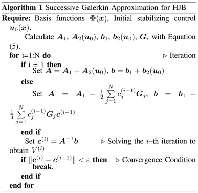
3. Successive Galerkin Approximation

A typical strategy to solve PDEs in numerical manner is Galerkin method [12]. Galerkin method approximates the solution with linear combination of finite number of trial functions.

[8] applied Galerkin method in sequential manner to obtain convergent solutions of HJB and HJI. Point-wise convergence of such method was also proved. Such approach was named Successive Galerkin Approximation (SGA). Although convergence and consistency under finite number of trial functions was not provided, with reasonable number and choice of trial (or basis) functions, it was verified that the feedback design through SGA performs decently. By taking the notations from [8], we summarize the SGA algorithm for HJB and HJI respectively in this section.

Let us begin by introducing the notations. For the basis functions $\left\{{\varphi }_1\mathrm{,}{\varphi }_2\mathrm{,}\cdots \mathrm{,}{\varphi }_N\right\}$, let $\Phi ={\left[\begin{array}{cccc}{\varphi }_1& {\varphi }_2& \cdots & {\varphi }_N\end{array}\right]}^{\text{T}}$. Now when the solution is approximated by $V\left(x\right)\approx c_1{\varphi }_1+\cdots +c_N{\varphi }_N$, let $c={\left[\begin{array}{cccc}{c}_1& c_2& \cdots & c_N\end{array}\right]}^{\text{T}}$. We further denote the integration region of Galerkin method by $\Omega$. Now we begin by introducing the iteration matrices for solution of the HJB.

$\begin{array}{l}{A}_1={\displaystyle {\int }_{\Omega }}\Phi \left(x\right)f{\left(x\right)}^{\text{T}}\cdot \nabla \Phi {\left(x\right)}^{\text{T}}\text{d}x\\ A_2\left(u_0\right)={\displaystyle {\int }_{\Omega }}\Phi \left(x\right)u_0{\left(x\right)}^{\text{T}}g{\left(x\right)}^{\text{T}}\cdot \nabla \Phi {\left(x\right)}^{\text{T}}\text{d}x\\ b_1=-{\displaystyle {\int }_{\Omega }}\mathcal{l}\left(x\right)\text{d}x\\ b_2\left(u_0\right)=-{\displaystyle {\int }_{\Omega }}{\Vert u_0\left(x\right)\Vert }_R^2\cdot \Phi \left(x\right)\text{d}x\\ G_i={\displaystyle {\int }_{\Omega }}\Phi {\frac{\partial {\varphi }_i}{\partial x}}^{\text{T}}g\left(x\right)R^{-1}g{\left(x\right)}^{\text{T}}\cdot \nabla \Phi \left(x\right)\text{d}x\mathrm{,}i=\mathrm{1,}\cdots \mathrm{,}N\end{array}$ (5)

The derivation of the above formulas (5) can be found at [8].

In Algorithm 1, $c^{\left(i-1\right)}$ is the result from the $\left(i-1\right)$ -th iteration and $\epsilon$ is the tolerance for termination criterion.

For solution of HJI, construction of the iteration matrices is as below.

$\begin{array}{l}{A}_1={\displaystyle {\int }_{\Omega }}\Phi \left(x\right)f{\left(x\right)}^{\text{T}}\cdot \nabla \Phi {\left(x\right)}^{\text{T}}\text{d}x\\ A_2\left(u_0\right)={\displaystyle {\int }_{\Omega }}\Phi \left(x\right)u_0{\left(x\right)}^{\text{T}}g{\left(x\right)}^{\text{T}}\cdot \nabla \Phi {\left(x\right)}^{\text{T}}\text{d}x\\ b_1=-{\displaystyle {\int }_{\Omega }}h{\left(x\right)}^{\text{T}}h\left(x\right)\cdot \Phi \text{d}x\\ b_2\left(u_0\right)=-{\displaystyle {\int }_{\Omega }}{\Vert u_0\left(x\right)\Vert }_R^2\cdot \Phi \left(x\right)\text{d}x\\ G_i={\displaystyle {\int }_{\Omega }}\Phi {\frac{\partial {\varphi }_i}{\partial x}}^{\text{T}}g\left(x\right)R^{-1}g{\left(x\right)}^{\text{T}}\cdot \nabla \Phi \left(x\right)\text{d}x\mathrm{,}i=\mathrm{1,}\cdots \mathrm{,}N\\ K_i={\displaystyle {\int }_{\Omega }}\Phi {\frac{\partial {\varphi }_i}{\partial x}}^{\text{T}}k\left(x\right)P^{-1}k{\left(x\right)}^{\text{T}}\cdot \nabla \Phi \left(x\right)\text{d}x\mathrm{,}i=\mathrm{1,}\cdots \mathrm{,}N\end{array}$ (6)

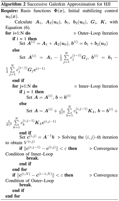
In Algorithm 2, $c^{\left(i\mathrm{,}j\right)}$ is the result from the $\left(i\mathrm{,}j\right)$ -th iteration, or the i-th inner loop and j-th outer loop iteration. $\epsilon$ is the tolerance for termination criterion. It was proved in the previous researches the convergence of both Algorithm 3 and Algorithm 3 for complete set of basis functions of continuous ${\mathcal{L}}_2$ space. But under finite number of basis functions, convergence of the solution procedure and convergence of the residual of the nonlinear PDE to zero was not proved. Due to finite computation resources, this is the case in practical applications. Our consequent results in this paper will review the results obtained from the SGA algorithms and point out such issues especially for the application in HJI case.

4. Problem Description

For illustrative purpose, we consider the gene regulatory network in cascaded form brought from [10]. The system dynamics $f\left(x\right)$ is represented by the below first order ODE. Though we specify the system dynamics as below, large amount of gene network systems are represented in the similar form and hence such an approach can be employed at various situations [10]. For the ${\mathcal{H}}_{\infty }$ -feedback control design of this system, linearization and application of fuzzy interpolation was attempted in [2].

$\begin{array}{l}{\stackrel{\dot{}}{x}}_1=4x_1^{0.5}-4x_1^{0.5}{x}_2^{-1}+1.5w\\ {\stackrel{\dot{}}{x}}_2=4x_1^{0.5}{x}_2^{-1}-2x_2^{0.5}-2x_2\\ {\stackrel{\dot{}}{x}}_3=2x_2^{0.5}-2x_3^{0.5}\\ {\stackrel{\dot{}}{x}}_4=2x_2-2x_4^{0.5}\end{array}$ (7)

where $w\left(t\right)$ is the external disturbance and the initial conditions are given by $x_1\left(0\right)=2.5$, $x_2\left(0\right)=2$, $x_3\left(0\right)=2$, $x_4\left(0\right)=2$. Such representation is also called the generalized-mass-action(GMA) form. It is evident that one equilibrium point is $x_e={\left[\begin{array}{cccc}1& 1& 1& 1\end{array}\right]}^{\text{T}}$. We sketch a formulaic design method of ${\mathcal{H}}_2$ and ${\mathcal{H}}_{\infty }$ -feedback controls for this system. Rewriting the Equation (2), it follows

${\frac{\partial V}{\partial x}}^{\text{T}}\left(f\left(x\right)+g\left(x\right)u\left(x\right)\right)+\mathcal{l}\left(x\right)+{\Vert u\Vert }_R^2=\frac{\text{d}}{\text{d}t}V\left(x\left(t\right)\right)+x^{\text{T}}Qx+{\Vert u\Vert }_R^2=0$ (8)

Because boundness of $V\left(x\right)$ has to be guaranteed for Galerkin’s approximation to be used, $\underset{t\to \infty }{lim}\frac{\text{d}}{\text{d}t}V\left(x\left(t\right)\right)=\underset{t\to \infty }{lim}-x^{\text{T}}Qx-{\Vert u\Vert }_R^2=0$. Hence it is evident that it is required to have $\underset{t\to \infty }{lim}x\left(t\right)=\underset{t\to \infty }{lim}u\left(t\right)=0$ for application of the SGA algorithm. Due to such reason, we consider the perturbed system as below.

$\begin{array}{l}{\stackrel{\dot{}}{\tilde{x}}}_1=4{\left({\tilde{x}}_1+1\right)}^{0.5}-4{\left({\tilde{x}}_1+1\right)}^{0.5}{\left({\tilde{x}}_2+1\right)}^{-1}+1.5w\\ {\stackrel{\dot{}}{\tilde{x}}}_2=4{\left({\tilde{x}}_1+1\right)}^{0.5}{\left({\tilde{x}}_2+1\right)}^{-1}-2{\left({\tilde{x}}_2+1\right)}^{0.5}-2\left({\tilde{x}}_2+1\right)\\ {\stackrel{\dot{}}{\tilde{x}}}_3=2{\left({\tilde{x}}_2+1\right)}^{0.5}-2{\left({\tilde{x}}_3+1\right)}^{0.5}\\ {\stackrel{\dot{}}{\tilde{x}}}_4=2\left({\tilde{x}}_2+1\right)-{\left(2{\tilde{x}}_4+1\right)}^{0.5}\end{array}$ (9)

By such perturbation, the system now has ${\tilde{x}}_e={\left[\begin{array}{cccc}0& 0& 0& 0\end{array}\right]}^{\text{T}}$ as an equilibrium point.

5. Numerical Demonstration & Discussion

In this section, we provide the numerical demonstration results of the previously described nonlinear gene network system. For both ${\mathcal{H}}_2$ and ${\mathcal{H}}_{\infty }$ -feedback designs, total six basis functions were used and are given by $\left\{{\varphi }_1,{\varphi }_2,{\varphi }_3,{\varphi }_4,{\varphi }_5,{\varphi }_6\right\}=\left\{{\tilde{x}}_1^2,{\tilde{x}}_2^2,{\tilde{x}}_3^2,{\tilde{x}}_1{\tilde{x}}_2,{\tilde{x}}_2{\tilde{x}}_3,{\tilde{x}}_1{\tilde{x}}_3\right\}$. Such choice was to obtain linear approximation of the true solution $u^{\mathrm{<mo>\; *\; </mo>}}\left(x\right)=-\frac{1}{2}{R}^{-1}{g}^{\text{T}}\frac{\partial V^{\mathrm{<mo>\; *\; </mo>}}}{\partial x}$ of HJB or HJI and satisfy $\underset{t\to \infty }{lim}u\left(x\left(t\right)\right)=0$ simultaneously. The integration region was set as $\left({\tilde{x}}_1\mathrm{,}{\tilde{x}}_2\mathrm{,}{\tilde{x}}_3\mathrm{,}{\tilde{x}}_4\right)\in \left[-\mathrm{0.3,3}\right]\times \left[-\mathrm{0.3,2}\right]\times \left[-\mathrm{0.3,2}\right]\times \left[-\mathrm{0.3,2}\right]$. For the feedback input, $g\left(x\right)={\left[\begin{array}{cc}{I}_2& O_2\end{array}\right]}^{\text{T}}$ was considered where $I_2$ and $O_2$ are the 2 × 2 identity and zero matrices respectively. Numerical simulation was done by Simulink software on Matlab 2019b with Macbook Pro, 2.4GHz Intel Core i5.

5.1. ${\mathcal{H}}_2$ -Feedback Design

For the design parameters, $Q=diag\left(\left[\begin{array}{cccc}10& 1& 1& 1\end{array}\right]\right)$ and $R=I_2$ was chosen. With the given basis, it took 7 iterations to converge within the tolerance $\epsilon ={10}^{-3}$. Converged solution is shown in Table 1. The state and control variables from the designed ${\mathcal{H}}_2$ controller are depicted in Figure 1. Simulation results with external disturbance entering through the state dynamics of ${\tilde{x}}_1$ are depicted in Figure 2 together with the random disturbance. The designed control system withstands such disturbance decently.

(a) State variables(b) Control variables

Figure 1. Time profiles of the state variables with the designed ${\mathcal{H}}_2$ -feedback: without external disturbance.

(a) State variables(b) Control variables(c) Applied External Disturbance

Figure 2. Time profiles of the state variables with the designed ${\mathcal{H}}_2$ -feedback: with external disturbance.

Table 1. Obtained solution of the HJB.

5.2. ${\mathcal{H}}_{\infty }$ -Feedback Design

For the ${\mathcal{H}}_{\infty }$ -feedback control design, as from [2], it is desirable to find the smallest $\gamma$ that the solution of HJI exists. Hence for the design parameter, $\gamma =3.5$ was used for the initial choice and we designed the feedback control throughout the solution. It took total 8 iterations for the outer loop to converge while inner loops typically took 4 iterations to converge within the same tolerance from previous subsection. Converged solution is shown in Table 2. Though the ${\mathcal{H}}_2$ feedback controller had shown slightly rapid convergence to the desired equilibrium point, both controllers show similar performances. Comparing with the results from [2] obtained from fuzzy interpolation after linearization, Figure 3 and Figure 4 show more rapid convergence. Such superiority of the feedback design without linearization was also confirmed at [9]. Then by trial and error, it was confirmed that the SGA algorithm also converges for smaller values of $\gamma \ge 0.4$. But for the solution obtained for $\gamma$ less than 2, the SGA algorithm did converge but the designed feedback controller exhibited unstable properties. Converged solution is shown in Table 3. Simulation results for $\gamma =1.0$ is depicted in Figure 5 and Figure 6 which shows unstable response regardless the presence of disturbance. We speculate that this is due to non-zero residual of the HJI (4). Because the choice of our basis was obviously not a complete set that can span the whole continuous ${\mathcal{L}}_2$ space, although the projection of the residual onto the subspace generated by our basis functions may be zero, it does not imply that the residual itself is zero. Regarding this, we would like to point out that the solution obtained from the SGA algorithm is indeed the utmost solution with the given basis, but it does not necessarily imply that it is the exact solution of HJI. This could be resolved through adding the number of basis functions or choosing appropriate basis functions depending on the system dynamics through heuristic. Though it was proposed in [8] a clever methodology exploiting tensor products to mitigate the computational burden of massive number of numerical integrations, in practice we are only allowed to use finite number of basis functions due to finite computing power. Also it should be pointed out that in a lot of cases, full-state observability of the system is not present and hence there are limitations in choice of basis functions too.

Table 2. Obtained solution of the HJI with $\gamma =3.5$.

(a) State variables(b) Control variables

Figure 3. Time profiles of the state variables with the designed ${\mathcal{H}}_{\infty }$ -feedback ( $\gamma =3.5$ ): without external disturbance.

(a) State variables(b) Control variables(c) Applied External Disturbance

Figure 4. Time profiles of the state variables with the designed ${\mathcal{H}}_{\infty }$ -feedback ( $\gamma =3.5$ ): with external disturbance.

(a) State variables(b) Control variables

Figure 5. Time profiles of the state variables with the designed ${\mathcal{H}}_{\infty }$ -feedback ( $\gamma =1.0$ ): without external disturbance.

Table 3. Obtained solution of the HJI with $\gamma =1.0$.

(a) State variables(b) Control variables(c) Applied External Disturbance

Figure 6. Time profiles of the state variables with the designed ${\mathcal{H}}_{\infty }$ -feedback ( $\gamma =1.0$ ): with external disturbance.

6. Conclusions & Future Scope

In this paper, nonlinear ${\mathcal{H}}_2$ and ${\mathcal{H}}_{\infty }$ -feedback controls have been developed for nonlinear gene regulatory network in GMA form. With the choice of basis functions from Section 5, Successive Galerkin Approximation did converge rapidly for both the Hamilton-Jacobi-Bellman and Hamilton-Jacobi-Isaacs equations. Because the majority of gene network systems are of the form of Equation (7), such feedback design methodology from this paper could be applied in a wide range of systems in GMA form. Comparison between the designed ${\mathcal{H}}_2$ and ${\mathcal{H}}_{\infty }$ -feedback control systems was made and for the hyper parameters used, it was confirmed that the two controllers exhibited similar performances.

It was also confirmed from our simulation that even when the SGA algorithm converged, there were cases where the corresponding feedback control system was unstable. This is due to nonzero residual of the HJI, and it needs to be further resolved by improvements in the algorithm for solving HJB and HJI. This issue could indeed be overcome by different choice of basis functions, but still there is no guarantee that the solution obtained with new basis functions will not exhibit such instability. Additionally in practice, there are limitations in observability of the state variables, which again impose restriction on the choice of the basis functions. Hence it requires further research to analyze the feedback control systems’ properties under finite number of basis functions to overcome these issues. Our consequent work will include breakthroughs in such issues discussed and consideration of stochastic disturbance entering through the system dynamics due to molecular noises.

Conflicts of Interest

The author declares no conflicts of interest regarding the publication of this paper.

References

[1]	Chen, B. and Chang, Y.-T. and Wang, Y.-C. (2008) Robust H∞-Stabilization Design in Gene Networks under Stochastic Molecular Noises: Fuzzy-Interpolation Approach. Systems, Man, and Cybernetics, Part B: Cybernetics, IEEE Transactions on, 38, 25-42.
[2]	Del Vecchio, D., Dy, A.J. and Qian, Y.L. (2016) Control Theory Meets Synthetic Biology. Journal of the Royal Society Interface, 13, Issue 120. https://doi.org/10.1098/rsif.2016.0380
[3]	Oudjama, F., Boumédiène, A., Messirdi, M. and Boubekeur, D. (2021) Comparison of Linear and Nonlinear H-Infinity Controllers for an Electric Vehicle Driven by the Permanent Magnet Synchronous Motor. International Journal on Emerging Technologies, 12, 247-257.
[4]	Fiore, G., Perrino, G., di Bernardo, M. and di Bernardo, D. (2016) In Vivo Real-Time Control of Gene Expression: A Comparative Analysis of Feedback Control Strategies in Yeast. ACS Synthetic Biology, 5, 154-162. https://doi.org/10.1021/acssynbio.5b00135
[5]	Fletcher, C.A.J. (1984) Computational Galerkin Methods. Springer, Berlin.
[6]	Modi, S., Dey, S. and Singh, A. (2021) Noise Suppression in Stochastic Genetic Circuits Using PID Controllers. PLOS Computational Biology, 17, e1009249. https://doi.org/10.1371/journal.pcbi.1009249
[7]	Volt, E.O. (2000) Computational Analysis of Biochemical Systems: A Practical Guide for Biochemists and Molecular Biologists. Cambridge Univ. Press, Cambridge.
[8]	Bea, R.W. (1998) Successive Galerkin Approximation Algorithms for Nonlinear Optimal and Robust Control. International Journal of Control, 71, 717-743. https://doi.org/10.1080/002071798221542
[9]	Saridis, G.N. and Lee, C.-S.G. (1979) An Approximation Theory of Optimal Control for Trainable Manipulators. IEEE Transactions on Systems, Man, and Cybernetics, 9, 1522-159. https://doi.org/10.1109/TSMC.1979.4310171
[10]	van der Schaft, A.J. (1992) L2-gain Analysis of Nonlinear Systems and Nonlinear State-Feedback H∞ Infinity Control. IEEE Transactions on Automatic Control, 37, 770-784. https://doi.org/110.1109/9.256331
[11]	Shannon, B., Zamora-Chimal, C.G., Postiglione, L., Salzano, D., Grierson, C.S., Marucci, L., Savery, N.J. and di Bernardo, M. (2020) In Vivo Feedback Control of an Antithetic Molecular-Titration Motif in Escherichia coli Using Microfluidics. ACS Synthetic Biology, 9, 2617-2624. https://doi.org/10.1021/acssynbio.0c00105
[12]	Zhang, W.H. and Chen, B. (2006) State Feedback H∞ Control for a Class of Nonlinear Stochastic Systems. SIAM Journal on Control and Optimization, 44, 1973-1991.