1. Introduction
One of the many problems that are considered to be NP-Hard is the Multiple Sequence Alignment one that initially requires, as for any other of its siblings, a specific encoding schema and design of the main functionalities of the heuristics algorithm being implemented and executed. This design was supported by references [1] [2] [3] and [4].
In a previous paper published during the ICeND2013 conference, we have discussed a generic encoding schema and some main methods that can be used in different heuristic algorithms for this particular problem, inspired by papers [5] [6] [7] and [8]. However, taken out of the entire research context, the remaining problem was the link between this encoding and the generic implementation of the main heuristics algorithms. In this paper, we’ll be discussing the implementation of the Genetic Algorithm, with some modifications, like a chronology traceability feature for further analysis and potential improvements, added to try to shorten the gap between the algorithm and the source that inspired it, which is none other than the structure and behavior of genome components.
2. Initial Algorithm
2.1. Standard Genetic Algorithm
Most Evolutionary Computing algorithms, including Genetic Algorithms, work iteratively on a subset of the solution space. We refer to this subset as a “population”. After the Initialization of the solution space, a Selection is made to choose two or more chromosomes (solutions, ex: phylogenetic trees) of the current POPULATION. These chromosomes, denoted as PARENTS, are subjected to a Crossover/Recombination operation, which consists of combining bits and pieces taken from 2 or more solutions to create as many solutions, called “offspring”. In their turn, the resulting OFFSPRING may be subjected to a Mutation process, which consists of slightly changing the solution. Both Crossover and Mutation operators are applied given certain respective probabilities. An individual Fitness Evaluation function is tested on each of the last operator’s results, which will be added to an INTERMEDIARY POPULATION refreshed per iteration. An Overall Evaluation goes through this new population, evaluating the whole population, by computing the fitness of the entire group. The intermediary population replaces the current one and the whole process is repeated until a termination criterion is met (for example: a certain number of iterations have elapsed). This idea was further supported by references [6] and [9] to [15].
Before stating the main steps of the standard algorithm, we would like to clarify the terminology used there:
- Solution = chromosome
- Population = set of solutions (chromosomes)
2.2. Main Procedure
The steps of the standard algorithm are as follows:
Initialize the population randomly.
Initialize to zero the number of generations to deal with
While NOT Terminate Process
Create a new empty population.
Do
Select two/more solutions to apply operators
Apply recombination between each pair of chromosomes
to get corresponding offspring, given a certain probability
Apply mutation to each offspring, given a certain probability
While (new population is not full)
Get fittest solution of the new population.
Compare it to the previous fittest global solution.
If (fitness value > that of the global one) Then
Update the fittest global solution
Set the new population as the current population
Increment number of generations
Return the fittest global solution found so far
We can see here that the structure of the solution is somewhat rigid obscuring or omitting the complexity of some properties of the input that might be useful for the optimization both structure wise and time wise.
Another main issue when working with the basic algorithm is the fact that it is a kind of black box, in the sense that even though the end result would be very satisfying we have no traceability on the values and performance of the algorithm which might go far from the optimal solution during one or more iterations, leaving us unable to analyze and help to tune some of the parameters.
3. Proposed Algorithm
Since Genetic Algorithms deal, in concept, with maximization, and since the suggested evaluation approach retrieves its values from a scoring (cost) matrix, the fitness function should be the negative of the evaluation function, as supported in references [6] to [14] inspiring the below suggested algorithm.
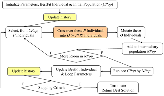
The steps of the below discussed algorithm are almost very similar to those of the basic standard algorithm, with the difference that some of them, highlighted in blue, offer the possibility to later on trace back each execution and allow better analysis, thus resulting in eventual update of initial parameters. The words/ fragments highlighted in green are more of structure enhancements that try to bridge the gap between genome composition and our genetic algorithm components structure.
3.1. Main Procedure
The steps of the algorithm implemented are as follows:
Initialize the population randomly.
Initialize to zero the number of generations to deal with
Select and backup the fittest global individual
Record in history the initial population & initialization
While NOT Terminate Process
Create a new empty population.
Do
Select two/more individuals to apply operators
Apply recombination between their {chromosomes, genes and/or
alleles}
to get offspring, given a certain probability.
Apply mutation to each individual of offspring, given a certain
probability
Save the newly generated individuals in the newly generated
population
While (new population is not full)
Get fittest individual of the new population.
Compare it to the previous fittest global individual.
If (fitness value > that of the global one) Then
Update the fittest global individual.
Set the new population as the current population
Increment number of generations
Record in history new population
Record in history new population generation time
Return the fittest global individual found so far
Even though crossover and mutation operators are applied given certain probabilities, it is very rare to find a parent individual (group of chromosomes) selected and passed to the new population without modification. The initial population is filled with a fixed number of individuals, whose chromosomes and genes are randomly generated. The fitness function of an individual is proportional evaluation of each of the chromosomes that individual includes. The algorithm supports elitism, to keep track of the best-fit individual found in previously handled and in the current population. It keeps on iterating and handling populations until the process termination criterion. In most problems, the termination criterion is satisfied when the algorithm reaches a certain number of generations.
Instead of focusing on speeding up the algorithm itself, we decided to attempt to work on the two main issues of the standard algorithm, proposing our own alternative or solution, by first “going back to the roots” that inspired the algorithm originally and give our algorithm the possibility to manage more granularly some properties of the input structure. This granularity brings with it the possibility for the algorithm to detect potential differences between evaluations due to the diverging effect of two properties previously merged together.
To support that point, let us consider a certain encoding of the parsimony problem discussed in the first reference of this paper. However, before looking at the problem from another perspective, let us highlight the post important encoding point: the solution is at the base composed of several leaf sequences, each of which is formed of a series of genetic code characters; which are then paired and linked to a parent (internal) sequence. This process continues until a single root node is reached.
Without flexibility, the default or preliminary evaluation encoding approach would be to cumulate the changes between characters at the same location of each of the pair nodes into one value for the pair, then into one value for the entire solution. Allowing the main operations of the algorithm to operate on the character level would allow evaluations of changes to be more accurate and help to gear the algorithm towards a better optimum. For instance, assuming that our local optimum would be around ATGATG, mutating ATCACAAG into ATGACAA might drive the algorithm closer to the fittest individual than ATCACAAG into ATCAGAAG, since moving C to G at the 3rd location would score higher than the same operation at the 5th location, as it will transcribe into a triplet closer to the one found in the parent.
While allowing specificity of granular data to help optimizing, we discovered the need to be able to recall previous runs, since making the algorithm display and/or interact with its designer would obviously be a worst option to consider. To avoid losing time at the expense of recording executions we opted to propose a simple straight forward approach to be consumed and implemented in a later stage, and most probably out of the real scope of this paper. While designing it, this functionality seemed to open up not only to improvements to the algorithm itself, but also to potential interaction with other components. Indeed, after running the standard algorithm many times, it remains a black box showing only the fittest solution at the end, no matter how much it goes closer to and away from the optimum found so far eating up resources.
Meanwhile, being able to retrace each run would give an edge to the designer of the algorithm to fine tune the parameters so that the next algorithm run would consume less resources and less time. In parallel, knowing when the algorithm was doing good and when it was doing worst can give the designer an edge to induce one or more functionalities allowing eventually other algorithms can join in and bring their added value into the table. At the same time, this ability can dig further towards letting the different operations being implemented/executed themselves using another algorithm to return a fair-enough optimal result.
3.2. Object Oriented Design
The below class diagram shows an overview of the interaction between the different classes instantiated during the runtime of the algorithm, discussed below. An allele can be found in at least one gene, which in turn may be part of one or more chromosomes. An individual can be described as a non-empty pool of chromosomes, which may or may not be related to each other. A population includes a fixed non-negative number of individuals, called the population size S.
As shown in Figure 1, the suggested flexible Genetic Algorithm tries to mimic as close as possible the genome as known in Biology. In other terms, each instance of an NP-problem, encoded to be used in this algorithm as an Individual, would be composed of one or more chromosomes. Each chromosome is constituted of a set of genes, which is defined as a combination of different alleles. In our parsimony phylogenetic problem, when dealing with DNA, we are consequently encoding each of the four {A, T, C, G} nucleotides into an allele. Therefore, a gene will encode a fixed group of DNA nucleotides.
This design makes the algorithm flexible, in a way that it allows changing the encoding schema by just modifying the design and implementation of alleles and genes according to the problem being handled. For instance, when dealing with binary encoding, an allele would have a value of “0” or “1”. For decimal encoding an allele value could be one of {“0”, “1”, “2”, “3”, “4”, “5”, “6”, “7”, “8”, “9”}. Moreover, a non-standard decimal encoding could give, for example, allele values between “00” and “79”.
Since the encoding can consider different alternatives of values for alleles, some methods that are problem-specific methods have to be implemented, among them: creating random genes, creating random chromosomes/individuals/ populations and their fitness functions, and handled by a sub-class of class “Nature”. The algorithm-dependent procedures (selection, recombination, mutation, termination) are handled by a sub-class of the “GeneticAlgorithm” class.
Going into further details in the class diagram, we can split the classes into 3 groups: the main generic classes dedicated to encoding problems (G1—as in Figure 2), the main generic GA class itself (G2—Figure 3) and the generic components used in the algorithm (G3—Figure 4).
The base “Nature” component represents the environment offering the possible {Individual, Chromosome, Gene} values and functionalities that the main
![]()
Figure 1.Suggested GA components diagram.
![]()
Figure 2.Suggested GA class diagram for G1.
![]()
Figure 3.Suggested GA class diagram for G2.
![]()
Figure 4.Suggested GA components class diagram for G3.
algorithm’s steps will be relying on to execute generic global and specific tasks. The other 5 classes are suggested base abstract implementations of the Nature component with purpose to handle common radix conversions instead of leaving them to each problem implementation.
In order to be mimicking as closely as possible the biology genome, the main GA algorithm attempts to manipulate these four components whereby the population is considered to be a set of individuals instead of a set of chromosome as handled by standard algorithms. Then, each individual is composed of a set of chromosomes, which in turn are considered to be a sequence of genes.
In order to be mimicking as closely as possible the biology genome, the main GA algorithm attempts to manipulate these four components whereby the population is considered to be a set of individuals instead of a set of chromosome as handled by standard algorithms. Then, each individual is composed of a set of chromosomes, which in turn are considered to be a sequence of genes.
This is the main algorithm offering both flexibility and execution tracing, by saving into current instance variables and some inherited properties a specific set of values per iteration while running.
One of the main reasons behind this distribution of components was also to allow the algorithm to work with a group of chromosomes as one block instead of separated, since in real-life chromosomes belonging to one individual don’t really crossover between them. However, during our researching, we discovered the topic of “jumping genes”, which relates in a few words to modifying chromosomes of an individual from a portion already existing on another from this same individual. This topic supports the need of having the suggested distribution of components.
Since we are talking about a generic implementation of the algorithm and its components, we implemented a few problems, as shown in Figure 5, that follow
![]()
Figure 5.Some supporting problem implementations.
the guidelines set by the above mentioned components diagrams but also by suggested encoding in reference paper 1, trying to cover different complexities. This set is divided into 3 groups relating all to a base class holding the math formulas: the first group is working with {2, 8, 10 and 16} radix applied to the default “Formula01” functionality; while the second group is a collection of problems handling different math formulas. The last group is the implementation of the encoding suggested in reference paper 1 about phylogenies.
In order to illustrate the generic implementations applied on these problems, we have developed a quick straight forward windows application, in which we dynamically modified the parameters a default algorithm based on the suggested generic implementation, instead of writing many versions inheriting for our main implementation.
The first step is to specify which problem the algorithm will work on, as per Figure 6. This list of problems is dynamically built from the set of problems including in the package, not only the one discussed above.
The second step would be to specify some of the properties required by both the Problem and the Algorithm, as shown in Figure 7 and Figure 8. Even though default values were given to those parameters, we advise to modify them to be able to view effective results.
The third and final step is to simply run the algorithm. In the above screenshot Figure 9, we are showing one population generated by the execution on problem Pb001, along with one of its individuals and consequently chromosomes and Genes. The next section of the screen shows the result of the execution leading to a fitness of −625, which is the best so far. If we were to run the algorithm for more time, this value will most probably change.
Figure 10 shows, as a graph, the progress of the algorithm run with the above parameters for 50 iterations, in other terms 50 populations were generated and evaluated. This graph shows that despite the simplicity of the problem Pb001
![]()
Figure 6.Win App, GA execution—problem selection.
![]()
Figure 7. Win App, GA execution problem parameterization.
![]()
Figure 8. Win App, GA execution algorithm parameterization.
![]()
Figure 9. Win App, GA execution—sample run.
![]()
Figure 10. Win App, GA execution—sample run graphs.
![]()
Figure 11. GA tracing functionality—binary nature.
formula and the algorithm having reached the best fit early, it kept on checking for a better one. Meanwhile, the time consumed seemed to stabilize with minor time “hiccups”.
Figure 11 illustrates the execution of the same algorithm run previously but on the binary problem implementation suggested earlier. Similar executions were done on the other radix implementations.
The last problem suggested and illustrated in Figure 12, was the implementation of the encoding suggested in reference paper 1 about phylogenies. For this, we added a functionality to decode and display any solution/individual and/or the result.
The third and final step is to simply run the algorithm. In the above screenshot Figure 9, we are showing one population generated by the execution on problem Pb001, along with one of its individuals and consequently chromosomes and Genes. The next section of the screen shows the result of the execution
![]()
Figure 12.GA tracing functionality—parsimony nature.
leading to a fitness of −625, which is the best so far. If we were to run the algorithm for more time, this value will most probably change.
4. Conclusions
This paper focused on the NP-Hard problem of finding an optimal tree topology where leaves represent biological sequences [1] [2]. The problem consists of minimizing the number of changes between given and/or derived sequences. As the number of sequences to be compared increases, the size of the search space grows exponentially. This fast growth induces the necessity of using optimization methods in order to come up with an acceptable optimal topology.
Since the phylogenetic trees literature have only discussed the use of an exact method (Fitch) or only one or at most two Heuristics (Genetic Algorithms, Simulated Annealing, Tabu Search, Simulated Evolution and Stochastic Evolution) in each one, with few of them having some pseudo-code/code or none what so ever, the entire research to which this paper belongs attempted to suggest an encoding schema ready to use in one or more of the above-mentioned algorithms, including the suggested alternatives.
This paper tried to propose a flexible traceable generic Genetic Algorithm so it can be used in other NP problems, not necessarily dealing with bio-informatics. The tracing/chronology property can be helpful essentially for detailed evaluation and analysis of the runs executed for the algorithms, with the corresponding encoding.
The research and this paper’s work can be extended by:
Applying benchmarks to validate the algorithms, and analyze more accurately the suggested algorithms’ generic alternatives.
References [16] - [23] come as a support to the need to Implementing the decoding functionality in a generic way, so that it might be applied to other problem implementations.
Attempting to resolve the below mentioned problems that appeared while researching the heuristics, whether the ones implemented, or the initial standard ones, are as follows:
➢ Fixed Input Parameters: which mean that there is a need to guess or write an algorithm to tune those parameters before running the algorithm itself.
® Algorithm requests a given number of generations, and population size, among others.
➢ Randomness doesn’t handle potentially repetitions:
® In both mutation & crossover methods.
➢ Initial solution may be far from the optimal one, thus the algorithm will take more time.
➢ Getting stuck with one procedure, even very close to a fairly acceptable solution. The use of a heuristic or fast algorithm might depend on the “distance” between the current solution and the optimal one, thus switching between algorithms might be helpful.