New Probability Distributions in Astrophysics: VIII. The Truncated Weibull—Pareto Distribution ()
1. Introduction
Regarding probability distributions, in recent years there have been many modifications of the standard distributions: here we analyze the case of the Weibull distribution. The Weibull distribution has two parameters, the scale and the shape, see [1] [2] [3]. The new Weibull-Pareto distribution (NWPD) has three parameters: the scale and two shapes, see [4] [5] [6], and allows modelling the flooding of the Wheaton river and bladder cancer [5], provides a way to design a multiple deferred state acceptance sampling plans for assuring the lifetime of products [7], the stress-strength model [8] and the breaking stress of carbon fibers [9]. Some generalizations of the NWPD have been suggested [10] [11] [12]. One example of a probability distribution in astrophysics is the lognormal distribution for the initial mass function (IMF), which allows modelling 8 young clusters [13]. Another example is the Schechter luminosity function (LF) for galaxies [14], which is currently used to model the absolute magnitude in catalogs of galaxies such as the 2dF Galaxy Redshift Survey (2dFGRS) [15], the Sloan Digital Sky Survey (SDSS) [16] and the Millennium Galaxy Catalogue (MGC) [17]. The previous two arguments allow exploring old and new probability distributions in order to understand which produces the best fit. At the time of writing, the effect of a truncation on the NWPD has not yet been explored, and therefore, after a review in Section 2, its effect on the NWPD will be explored in Section 3. Section 4 is devoted to the derivation of the luminosity function for galaxies using both the regular and truncated versions, and then Section 5 is devoted to the astrophysical applications, such as the initial mass function for stars, the photometric maximum of the number of galaxies and the average absolute magnitude for galaxies.
2. The Weibull—Pareto Distribution
Let X be a random variable defined on
; the two-parameter Weibull distribution function (DF),
, is
(1)
where b and c, both positive, are the scale and the shape parameters, see [18]. The NWPD is also defined on
:
(2)
where a is a new positive shape parameter and the PDF, f, is
(3)
Careful attention should be paid to the fact that the transformation
(4)
in Equation (2) followed by
transforms the NWPD DF into the Weibull DF.
The statistical parameters can be parametrized by introducing the following function
(5)
where
(6)
is the gamma function, see [19].
The average value or mean,
, is
(7)
the variance,
, is
(8)
the skewness is
(9)
and the kurtosis
(10)
The rth moment about the origin for the NWPD,
, is
(11)
where r is an integer. The median is at
(12)
and the mode is at
(13)
Random generation of the NWPD variate X is given by
(14)
where R is the unit rectangular variate. One method to derive the three parameters a, b and c is to numerically solve the three following equations which arise from the maximum likelihood estimator (MLE)
(15a)
(15b)
(15c)
where the
are the elements of the experimental sample with i varying between 1 and n. Another method to derive the parameters is to introduce the moments of the experimental sample
(16)
The three parameters can then be found by solving the following three non-linear equations (the method of moments)
(17a)
(17b)
(17c)
Figure 1 reports the influence of the second shape parameter, a, of the NWPD on the Weibull distribution.
3. The Truncated Weibull—Pareto Distribution
The right and left truncated NWPD, see Equation (3), is defined on
and has PDF
(18)
where a, b, c,
and
are positive parameters and DT means double truncation. The DF is
(19)
The average is
![]()
Figure 1. NWPD PDF with
,
with
(red line), with
(green line) and with
(blue line).
(20)
where
is the Whittaker M function, see [19]. The variance exists but has a complicated expression. The rth moment about the origin for the truncated NWPD is
(21)
The median is at
(22)
and the mode is at the same value of the NWPD, see Equation (13). The random generation of the truncated NWPD variate X is given by
(23)
The two parameters
and
are here assumed to be the minimum and the maximum of the experimental sample. The remaining three parameters, a, b and c, can be determined by numerically solving the three following equations which arise from the MLE
(24)
(25)
(26)
where the
are the elements of the experimental sample with i varying between 1 and n.
4. Luminosity Function for Galaxies
In this section we derive the luminosity function for galaxies (LF) using both the regular and truncated DFs.
4.1. Using the Regular DF
In order to derive the NWPD LF, we start from the PDF as given by Equation (3),
(27)
where L is the luminosity defined for
,
is the characteristic luminosity and
is a normalization, i.e. the number of galaxies in a cubic Mpc. We now introduce the following useful formulae relating the absolute magnitude and luminosity
(28)
where
and
are the luminosity and absolute magnitude of the sun in the considered band. The LF in absolute magnitude is therefore
(29)
4.2. Using the Truncated DF
The truncated NWPD LF for galaxies according to Equation (18) is
(30)
where the random variable L is defined for
,
is the lower boundary in luminosity,
is the upper boundary in luminosity,
is the characteristic luminosity and
is the normalization. The magnitude version is
(31)
where M is the absolute magnitude,
is the characteristic magnitude,
is the lower boundary of the magnitudes and
is the upper boundary of the magnitudes. The two luminosities
and
are connected with the absolute magnitudes
and
through the following relation:
(32)
where the indices u and l are inverted in the transformation from luminosity to absolute magnitude. The mean theoretical absolute magnitude,
, can be evaluated as
(33)
5. Astrophysical Applications
In this section, we review the adopted statistics and we apply the truncated NWPD to: the initial mass function for stars (IMF), which is often modeled by the lognormal distribution [20]; the LF for galaxies, which is usually modeled by the Schechter LF [14]; the photometric maximum for galaxies, which is modeled by the Schechter LF and the generalized gamma LF [21]; and the mean absolute magnitude for galaxies, which at the moment of writing has not yet been modelled by a probability distribution.
5.1. Statistics
The merit function
is computed according to the formula
(34)
where n is the number of bins,
is the theoretical value, and
is the experimental value represented by the frequencies. The theoretical frequency distribution is given by
(35)
where N is the number of elements of the sample,
is the magnitude of the size interval, and
is the PDF under examination. A reduced merit function
is given by
(36)
where
is the number of degrees of freedom, n is the number of bins, and k is the number of parameters. The goodness of the fit can be expressed by the probability Q, see equation 15.2.12 in [22], which involves the number of degrees of freedom and
. According to [22] p. 658, the fit “may be acceptable” if
. The Akaike information criterion (AIC), see [23], is defined by
(37)
where L is the likelihood function and k the number of free parameters in the model. We assume a Gaussian distribution for the errors. Then the likelihood
function can be derived from the
statistic
where
has been computed by Equation (34)), see [24] [25]. Now the AIC becomes
(38)
The Kolmogorov-Smirnov test (K-S), see [26] [27] [28], does not require binning the data. The K-S test, as implemented by the FORTRAN subroutine KSONE in [22], finds the maximum distance, D, between the theoretical and the astronomical CDFs as well as the significance level
, see Formulas (14.3.5) and (14.3.9) in [22]; if
, the goodness of the fit is believable.
5.2. The IMF for Stars
The first test is performed on NGC 2362 where the 271 stars have a range
, see [29] and CDS catalog J/MNRAS/384/675/table 1. The second test is performed on the low-mass IMF in the young cluster NGC 6611, see [30] and CDS catalog J/MNRAS/392/1034. This massive cluster has an age of 2 - 3 Myr and contains masses from
. Therefore the brown dwarfs (BD) region,
is covered. The third test is performed on the
Velorum cluster where the 237 stars have a range
, see [31] and CDS catalog J/A + A/589/A70/table 5. The fourth test is performed on the young cluster Berkeley 59 where the 420 stars have a range
, see [32] and CDS catalog J/AJ/155/44/table 3. The results are presented in Table 1 for the truncated NWPD with three parameters, where the last column reports whether the results are better compared to the Weibull distribution (Y) or worse (N).
As an example, the empirical PDF visualized through histograms as well as the theoretical PDF for NGC 2362 and NGC 6611 are reported in Figure 2 and in Figure 3 respectively.
![]()
Figure 2. Empirical PDF of the mass distribution for NGC 2362 (271 stars) (red histogram) with a superposition of the truncated NWPD (green dotted line). Theoretical parameters as in Table 1.
![]()
Table 1. Numerical values of
, AIC, probability Q, D, the maximum distance between theoretical and observed DF, and
, significance level, in the K-S test of the truncated NWPD with three parameters for different mass distributions. The last column (W) indicates an AIC lower (Y) or higher (N) than that for the Weibull distribution with two parameters. The number of linear bins, n, is 20.
![]()
Figure 3. Empirical PDF of the mass distribution for young cluster NGC 6611 (207 stars) (red histogram) with a superposition of the truncated NWPD (green dotted line). Theoretical parameters as in Table 1.
5.3. The LF for Galaxies
We now perform the same test as in Section 5.3 in [33]. The Schechter function, the NWPD LF represented by Formula (29) and the data are reported in Figure 4, parameters as in Table 2.
A careful examination of Table 2 reveals that the NWPD LF has a lower
than for the Schechter LF. Figure 5 reports the LF for QSO in the case
, see [34], with parameters as reported in Table 3.
5.4. The Photometric Maximum
In the pseudo-Euclidean universe, we introduce
(39)
which allows defining the joint distribution in z (redshift) and f (flux) for NPWD LF as
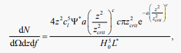 (40)
(40)
where
,
and
represent the differentials of the solid angle, the redshift, and the flux, respectively,
is the characteristic luminosity,
is the speed of light, and
is the Hubble constant; see [33] for more details. The solution of the following non-linear equation determines a maximum at
(41)
An analytical result can be obtained by computing a truncated multivariate
![]()
Figure 4. The LF data of SDSS (
) are represented with error bars. The continuous line fit represents the NWPD LF (29) and the dotted line represents the Schechter function.
![]()
Figure 5. The observed LF for QSOs, empty stars with error bar, and the fit by the NWPD LF for z in
and M in
. Parameters as in Table 3.
![]()
Table 2. Numerical values and
of the LFs applied to SDSS Galaxies in the
band.
![]()
Table 3. Parameters of the NWPD LF for QSOs in the range of redshift
when
and
.
Taylor series expansion of Equation (41), with respect to the variables z and a, to order n. As an example, when
,
and
, we have the following approximate equation which defines the photometric maximum as a function of a and b
(42)
Figure 6 reports the approximate solution to the third order (
,
,
) of the photometric maximum which can be found selecting the positive solution of an algebraic equation of second degree.
Figure 7 reports a comparison of the truncated multivariate Taylor series and the numerical solution.
A numerical result is reported in Figure 8 where we display the number of observed galaxies for the 2 MASS Redshift Survey (2 MRS) catalog at a given apparent magnitude and both the Schechter and the NWPD models for the number of galaxies as functions of the redshift. The theoretical parameters of the two curves in the above figure are chosen so as to minimize
. One distribution (the full line) gives a better fit to the data at lower redshift than the other (the dashed line), while for the higher redshift, the opposite is true.
![]()
Figure 6. Approximate positive solution of the photometric maximum in units of
when
,
and
as a function of the parameters a and b.
![]()
Figure 7. Approximate positive solution of the photometric maximum in units of
(
,
,
) as a function of the parameters a (blue dotted line) and numerical solution (red full line).
![]()
Figure 8. The galaxies of the 2 MRS with
or
are organized in frequencies versus heliocentric redshift, (empty circles); the error bar is given by the square root of the frequency. The maximum frequency of observed galaxies is at
. The full line is the theoretical curve generated by
as given by the application of the Schechter LF which is Equation (43) in [35] and the dashed line represents the NWPD LF which is Equation (40). The NWPD LF parameters are
,
,
,
for the Schechter LF and
for the NWPD LF.
5.5. Mean Absolute Magnitude
We review the most important equations that allow modelling the mean absolute magnitude as a function of the redshift. The absolute magnitude is
(43)
where
for the 2 MRS catalog.
The theoretical average absolute magnitude of the truncated NWPD LF, see Equation (33), can be compared with the observed average absolute magnitude of the 2 MRS as a function of the redshift. To fit the data, we assumed the following empirical dependence on the redshift for the characteristic magnitude of the truncated NWPD LF
(44)
where
and
are the minimum and the maximum value of the redshift in the considered catalog, in the case of the 2 MRS catalog
and
. The lower bound in absolute magnitude is given by the minimum magnitude of the selected bin, the upper bound is given by Equation (43), the characteristic magnitude varies according to Equation (44) and Figure 9 shows a comparison between the theoretical and the observed absolute magnitude for the 2 MRS catalog.
![]()
Figure 9. Average absolute magnitude of the galaxies belonging to the 2 MRS (green-dashed line), theoretical average absolute magnitude for the truncated NWPD LF (blue dash-dot-dash-dot line) as given by Equation (33) with
and
, lower theoretical curve as represented by Equation (43) (red line) and minimum absolute magnitude observed (cyan dotted line).
6. Conclusions
The truncated Weibull-Pareto distribution. We derived the PDF, the DF, the average value, the rth moment, the median and an expression to generate random variates. The three parameters, a, b and c are derived by the MLE or by the method of moments for the truncated Weibull-Pareto distribution.
Quality of fits
The third parameter a of the NWPD adds flexibility to the usual Weibull distribution and as an example, Table 1 reports the parameters for four samples of stars, but due to Formula (4) the reduced
is not lower than those for the Weibull distribution.
Weibull—Pareto luminosity function
The NWPD LF in the absolute magnitude version is derived using the standard and the truncated DFs, see Formulas (29) and (31). The application to both the SDSS Galaxies and to the QSOs in the range of redshift
yields a lower reduced merit function than that from using the Schechter LF, see Table 2 and Figure 5.
Cosmological applications
The maximum in the number of galaxies for a given solid angle as a function of the redshift which is visible in the catalog of galaxies can be modeled with the NWPD LF, see Figure 8. The average absolute magnitude of the 2 MRS galaxies as a function of the redshift, can be theoretically modeled with the truncated NWPD LF, see Figure 9.