Communication-Censored Distributed Learning for Stochastic Configuration Networks

Yujun Zhou, Xiaowen Ge, Wu Ai^*

College of Science, Guilin University of Technology, Guilin, China.

DOI: 10.4236/ijis.2022.122003                

Abstract

This paper aims to reduce the communication cost of the distributed learning algorithm for stochastic configuration networks (SCNs), in which information exchange between the learning agents is conducted only at a trigger time. For this purpose, we propose the communication-censored distributed learning algorithm for SCN, namely ADMMM-SCN-ET, by introducing the event-triggered communication mechanism to the alternating direction method of multipliers (ADMM). To avoid unnecessary information transmissions, each learning agent is equipped with a trigger function. Only if the event-trigger error exceeds a specified threshold and meets the trigger condition, the agent will transmit the variable information to its neighbors and update its state in time. The simulation results show that the proposed algorithm can effectively reduce the communication cost for training decentralized SCNs and save communication resources.

Keywords

Event-Triggered Communication, Distributed Learning, Stochastic Configuration Networks (SCN), Alternating Direction Method of Multipliers (ADMM)

1. Introduction

In traditional machine learning, it is generally assumed that the whole dataset is located at a single machine. However, in the big data environment, the massiveness and incompleteness of big data make single-threaded optimization algorithms face huge challenges that are difficult to solve. Therefore, parallel optimization and learning algorithms using shared-nothing architectures have been proposed, such as MapReduce [1], by dividing sample data and model parameters, using multi-threaded methods to train sub-dataset in parallel. The model parameters are updated in a shared memory [2]. However, it is impossible to collect data centrally for calculations on one machine sometimes. Data may need to be communicated between different machines [3], and the amount of data stored by one machine is limited after all. To solve the problem of distributed data storage and limited computation, a better way is to process data in a distributed environment, which leads to distributed learning algorithms.

Distributed learning is to use the same algorithm to train data distributed on multiple agents connected in a network and coordinate the state of each agent through neighboring communication to jointly obtain a consistent value, to achieve the effect close to the centralized training and learning on the whole dataset [4]. A general framework for training neural networks by distributed methods is summarized in the work of [5]. Generally speaking, in the distributed learning algorithm, a large amount of information communication between nodes on the network is required to achieve the purpose of cooperation. As the network scale increases, the communication load between network nodes may be unbearable. Especially in an environment with limited resources, redundant communications can increase the computational load and communication. The energy consumed by communication between nodes is much greater than the energy consumed by calculations [6]. In the case of limited energy resources, how to reduce the frequency of communication to obtain better system performance is an important topic of current research. This leads to an event-triggered communication mechanism. The concept of event-triggered control was introduced in [7]. The main idea is that information is transmitted between agents only when they are in extraordinary need [8]. Distributed event-triggered control has been developed in the present. [9] discusses the event-triggered consensus problem, applying event-triggered control to the multi-agent consensus problem. Model-based edge-event-triggered mechanisms in a directed communication topology were investigated in [10]. In the context of distributed coordination control, dynamic event-triggered control was first introduced [11].

Event-triggered control was originally a control method in the field of industrial control. In the process of data transfer between controllers, sensors and actuators, the updates of the controller output are mostly constant sampling with equal cycles. However, when a system is expected to run smoothly without external interference or less interference if the control tasks are still performed periodically at this time, this conservative control method may cause a heavy load on the communication and the controller. And even cause problems such as data congestion and delay. Therefore, in order to alleviate the shortcomings of the periodic sampling method, many researchers began to study event-triggered control, which is considered to be an effective alternative to the periodic sampling control method. Compared with the traditional periodic sampling control method, event-triggered control can effectively reduce the computational load and reduce the amount of communication.

Up to now, various trigger schemes have been proposed to improve communication efficiency. For the first time, Dimarogonas et al. used event-triggered control in the cooperative research of multi-agent systems. Under centralized and distributed control strategies, they designed event-triggered functions based on state dependence, and obtained corresponding event-triggered time series, getting two event-triggered methods. One is the centralized event-triggered control method [12]. This method requires all nodes to know the global information of the network, and also requires all nodes to update their control signals at the same time, that is, events occur at all nodes at the same time. The other is a distributed event-triggered control method [13]. According to this method, all nodes need to constantly access the state of neighboring nodes to determine when to update their state parameters. However, these requirements may be difficult to meet in practice. This paper mainly studies distributed event-triggered control based on state dependence.

This paper aims to introduce an event-triggered communication mechanism into the distributed learning algorithm based on stochastic configuration networks (SCN) to improve the distributed learning algorithm. Only when each node and its neighboring nodes on the network topology are in great need, information will be transmitted between them. By designing a trigger function and continuously monitoring the parameters, only when the error of the node parameters exceeds the threshold to meet the trigger function conditions, the node will transmit the variable information to its neighbors and update its variable information in time. Finally, achieve the purpose of effectively reducing the communication volume of distributed learning algorithms.

2. Related Works

2.1. Notation

For matrices $A\in {ℝ}^{a\times n}$ and $B\in {ℝ}^{b\times n}$, $\left[A\mathrm{<mo>\; ;\; </mo>}B\right]\in {ℝ}^{\left(a+b\right)\times n}$ is represented as stacking two matrices by row. $\langle v_1\mathrm{,}{v}_2\rangle \mathrm{<mo>\; :\; </mo>}=v_1^{\text{T}}{v}_2$ as the inner product of $v_1$ and $v_2$, the Euclidean normal form $\Vert v\Vert \mathrm{<mo>\; :\; </mo>}=\sqrt{\langle v\mathrm{,}v\rangle }$ of vector v is naturally derived. In the whole paper, network topology $\mathcal{G}\left(\mathcal{V}\mathrm{,}\mathcal{E}\mathrm{,}A\right)$, where $\mathcal{E}=\left\{\mathrm{1,}\cdots \mathrm{,}M\right\}$ is a set of M directed arcs and $A=\left[a_{ij}\right]\in {ℝ}^{V\times V}$ is adjacency matrix, the elements $a_{ij}$ in the matrix represent the degree of association between a node i and another node j, if $\left(j\mathrm{,}i\right)\in \mathcal{E}$, then $a_{ij}>0$, otherwise $a_{ij}>0$. The degree matrix is defined as $D=\text{diag}\left\{{\displaystyle {\sum }_{j\in {\mathcal{N}}_i}}{a}_{ij}\right\}\in R^{N\times N}$. Furthermore, the arc source matrix of expansion block is defined as $A_s\in {ℝ}^{Mp\times V_p}$, which contains $M\times V$ square blocks ${\left(A_s\right)}_{e\mathrm{,}i}\in {ℝ}^{p\times p}$. If arc $e=\left(i\mathrm{,}j\right)\in \mathcal{E}$, then ${\left(A_S\right)}_{e,i}=I_p$, otherwise it is an empty set. Similarly, the extended block arc objective matrix $A_d\in {ℝ}^{Mp\times V_p}$ is defined, where ${\left(A_d\right)}_{e\mathrm{,}i}\in {ℝ}^{p\times p}$ is not an empty set but $I_p$ if and only if arc $e=\left(i\mathrm{,}j\right)\in \mathcal{E}$ points to node j. Then, the extended directional incidence matrix is defined as $G_o=A_s-A_d$, the undirected incidence matrix is defined as G_u = A_s + A_d, the directed Laplacian is denoted as $L_o=\frac{1}{2}{G}_o^{\text{T}}{G}_o$, and the undirected Laplacian is denoted as $L_u=\frac{1}{2}{G}_u^{\text{T}}{G}_u$.

2.2. Alternating Direction Method of Multipliers (ADMM)

ADMM is a powerful tool to solve structured optimization problems with two variables. These two variables are separable in the loss function and constrained by linear equality. By introducing Lagrange multiplier, the optimization problem with n variables and k constraints can be transformed into an unconstrained optimization problem with $n+k$ variables.

It can be used to solve the unconstrained and separable convex optimization problem with fixed topology in a communication network

$x^{*}=\underset{x}{\arg \min }f\left(x\right)=\underset{x}{\arg \min }{\displaystyle \underset{i=1}{\overset{V}{\sum }}}{f}_i\left(x\right).$ (1)

The problem can be rewritten as a standard bivariate form, by introducing the copy of global variable $x^{\mathrm{<mo>\; *\; </mo>}}$, local variable $x_i\in {ℝ}^p$ and auxiliary variable $z_{ij}\in {ℝ}^p$ at node i. Since the network is connected, the problem (1) is equivalent to the following bivariate form:

$\begin{array}{ll}\underset{\left\{x_i\right\}\mathrm{,}\left\{z_{ij}\right\}}{\min }\hfill & {\displaystyle \underset{i=1}{\overset{V}{\sum }}}{f}_i\left(x_i\right)\hfill \\ \text{s}\text{.t}\text{.}\hfill & x_i=z_{ij}\mathrm{,}{x}_j=z_{ij}\mathrm{,}\forall \left(i\mathrm{,}j\right)\in \mathcal{A}\mathrm{.}\hfill \end{array}$ (2)

The kernel optimal solution satisfies $x_i^{*}=x^{*}$ and $z_{ij}^{*}=x^{*}$, where $x^{\mathrm{<mo>\; *\; </mo>}}$ is the global optimal solution of the problem (1). By concatenating variables to obtain $x=\left[x_1\mathrm{<mo>\; ;\; </mo>}\cdots \mathrm{<mo>\; ;\; </mo>}{x}_V\right]\in {ℝ}^{V_p}$ and $z=\left[z_1\mathrm{<mo>\; ;\; </mo>}\cdots \mathrm{<mo>\; ;\; </mo>}{z}_m\right]\in {ℝ}^{mp}$, and introducing the global function $f\left(x\right):={\displaystyle {\sum }_{i=1}^V}{f}_i\left(x_i\right)$ to express $A:=\left[A_s;A_d\right]\in {ℝ}^{2mp\times V_p}$ and $B:=\left[-I_{mp};-I_{mp}\right]$, the matrix form of problem (2) can be changed to

$\begin{array}{ll}\underset{x\mathrm{,}z}{{\displaystyle \min }}\hfill & f\left(x\right)\mathrm{,}\hfill \\ \text{s}\text{.t}\text{.}\hfill & Ax+Bz=0.\hfill \end{array}$ (3)

The augmented Lagrangian function of problem (3) is introduced

$L\left(x\mathrm{,}z\mathrm{,}\lambda \right)=f\left(x\right)+\langle \lambda \mathrm{,}Ax+Bz\rangle +\frac{\rho }{2}{\Vert Ax+Bz\Vert }^2\mathrm{.}$

A penalty parameter $\rho$ is a normal number, Lagrange multiplier $\lambda \mathrm{<mo>\; :\; </mo>}=\left[\varphi \mathrm{<mo>\; ;\; </mo>}\psi \right]\in {ℝ}^{2mp}$. Then, in the $k+1$ iteration, the update of parameters is

$\begin{array}{l}{x}^{k+1}=\arg \underset{x}{\min }L\left(x,z^k,{\lambda }^k\right),\\ z^{k+1}=\arg \underset{z}{\min }L\left(x^{k+1},z,{\lambda }^k\right),\\ {\lambda }^{k+1}={\lambda }^k+\rho \left(A{x}^{k+1}+B{z}^{k+1}\right).\end{array}$ (4)

When variables ${\varphi }^0=-{\psi }^0$ and $G_u{x}^0=2z^0$ are initialized, $z^{k+1}$ can be eliminated and ${\lambda }^{k+1}$ can be replaced by a low dimensional dual variable $\mu$, so that (4) the variables will be updated as follows

$x_i^{k+1}=\arg \underset{x_i}{\min }\left\{f_i\left(x_i\right)+\langle x_i,{\mu }_i^k-\rho {\displaystyle \underset{j\in N_i}{\sum }}\left(x_i^k+x_j^k\right)\rangle +\rho d_{ii}{\Vert x_i\Vert }^2\right\},$ (5)

${\mu }_i^{k+1}={\mu }_i^k+\rho {\displaystyle \underset{j\in N_i}{\sum }}\left(x_i^{k+1}-x_j^{k+1}\right).$ (6)

The unconstrained and separable optimization problem in (1) can be solved through continuous iterations.

2.3. Stochastic Configuration Network (SCN)

The SCNrandomly assigns the hidden layer parameters within an adjustable interval and introduce a supervised mechanism to ensure its infinite approximation property. As an incremental learning algorithm, SCN builds a pool of candidate nodes to select the best node in each incremental learning process, which accelerates the convergence speed. Given N training set samples ${\left\{\left(x_n\mathrm{,}{t}_n\right)\right\}}_{n=1}^N$, the input vector is $X=\left\{x_1\mathrm{,}\cdots \mathrm{,}{x}_N\right\}$, and the corresponding output is $T=\left\{t_1\mathrm{,}\cdots \mathrm{,}{t}_N\right\}$. The SCN model with $L-1$ hidden layer nodes can be expressed as:

$f_{L-1}\left(x\right)={\displaystyle \underset{l=1}{\overset{L-1}{\sum }}}{\beta }_l{g}_l\left(x\mathrm{,}{w}_l\mathrm{,}{b}_l\right)\mathrm{,}l=\mathrm{1,2,}\cdots \mathrm{,}L-\mathrm{1,}$ (7)

where $g\left(x\right)$ as activation function and $\beta ={\left[{\beta }_1\mathrm{,}\cdots \mathrm{,}{\beta }_{L-1}\right]}^{\top }\in {ℝ}^{\left(L-1\right)\times M}$ is the output weight. The residual error, that is, the difference between the actual observation value and the fit value can be expressed:

$e_{L-1}\left(x\right)=f\left(x\right)-f_{L-1}\left(x\right)\mathrm{.}$ (8)

If $\Vert e_{L-1}\Vert$ does not reach the target value, it generates a new $g_L$, and the output weight ${\beta }_L$ is also recalculated as:

$f_L\left(x\right)=f_{L-1}\left(x\right)+{\beta }_L{g}_L\left(x\right)\mathrm{.}$ (9)

The incremental construction learning algorithm is an effective method to solve the network structure, starting from randomly generating the first node, and gradually adding nodes to the network. According to the general approximation property already proved in [14], given span( $\Gamma$ ) is dense in $L_2$ and for any $g\in \Gamma ,\Vert g\Vert <b_{\varphi }$ where $b_g\in {ℝ}^{+}$ when adding a new node, the new input weights and deviations are subject to the following inequalities:

${\langle e_{L-\mathrm{1,}q}\mathrm{,}{g}_L\rangle }^2\ge b_g^2{\delta }_{L\mathrm{,}q}\mathrm{,}q=\mathrm{1,}\cdots \mathrm{,}M\mathrm{,}$ (10)

where ${\delta }_{L\mathrm{,}q}=\left(1-r-{\mu }_L\right){\Vert e_{L-\mathrm{1,}q}\Vert }^2$, ${\mu }_L=\left(1-r\right)/\left(L+1\right)$, $0<r<1$. The optimization problem for the output weights can be obtained by the following equation:

${\left[{\beta }_1^{\mathrm{<mo>\; *\; </mo>}}\mathrm{,}{\beta }_2^{\mathrm{<mo>\; *\; </mo>}}\mathrm{,}\cdots \mathrm{,}{\beta }_L^{\mathrm{<mo>\; *\; </mo>}}\right]}^{\top }=\underset{\beta }{\arg \min }\Vert f-{\displaystyle \underset{l=1}{\overset{L}{\sum }}}{\beta }_l{g}_l\Vert \mathrm{,}$ (11)

where $f_L^{\mathrm{<mo>\; *\; </mo>}}={\displaystyle {\sum }_{l=1}^L}{\beta }_l^{\mathrm{<mo>\; *\; </mo>}}{g}_l$ and ${\beta }_l^{\mathrm{<mo>\; *\; </mo>}}={\left[{\beta }_{l\mathrm{,1}}^{\mathrm{<mo>\; *\; </mo>}}\mathrm{,}{\beta }_{l\mathrm{,2}}^{\mathrm{<mo>\; *\; </mo>}}\mathrm{,}\cdots \mathrm{,}{\beta }_{l\mathrm{,}M}^{\mathrm{<mo>\; *\; </mo>}}\right]}^{\top }$.

3. Distributed Event-Triggered Learning for SCN

For a distributed learning algorithm, it will impose a consistency constraint on the consistency of each node, making the final solution effect close to that of the centralized processing approach. In the centralized SCN model, the output weights $\beta$ can be obtained by the following equation [15]:

$\begin{array}{ll}\underset{\beta \mathrm{,}\left\{{\xi }_n\right\}}{\min }\hfill & \frac{C}{2}{\Vert \beta \Vert }^2+\frac{1}{2}{\displaystyle \underset{n=1}{\overset{N}{\sum }}}{\Vert {\xi }_n\Vert }^2\hfill \\ \text{s}\text{.t}\text{.}\hfill & {\beta }^{\top }g\left(x_n\right)=t_n^{\top }-{\xi }_n^{\top }\mathrm{,}n=\mathrm{1,}\cdots \mathrm{,}N\mathrm{,}\hfill \end{array}$ (12)

where ${\xi }_n$ is the training error corresponding to the input vector and $C>0$ regularization parameter. Bring the constraint conditions to (12) we can obtain

$\underset{\beta }{\min }\frac{C}{2}{\Vert \beta \Vert }^2+\frac{1}{2}{\Vert H\beta -T\Vert }^2\mathrm{,}$ (13)

where the hidden layer output matrix is written as H and the target output matrix is denoted by T, i.e.,

$H=\left[\begin{array}{c}{g}^{\top }\left(x_1\right)\\ ⋮\\ g^{\top }\left(x_N\right)\end{array}\right]\mathrm{,}T=\left[\begin{array}{c}{t}_1^{\top }\\ ⋮\\ t_N^{\top }\end{array}\right]\mathrm{.}$ (14)

SCN is placed in a distributed computing scenario where the training samples are to be written ${\mathcal{S}}_i={\left\{\left(x_{n\mathrm{,}i}\mathrm{,}{t}_{n\mathrm{,}i}\right)\right\}}_{n=1}^{N_i}$ and each agent $i\in \mathcal{V}$ on the network topology has its own local dataset, the input vector can be denoted as $x_{n\mathrm{,}i}\in {ℝ}^D$, and the corresponding output vector is denoted as $t_{n\mathrm{,}i}\in {ℝ}^M$. We want to train all the training sets ${\mathcal{S}}_i$ using a distributed approach, then we can turn the problem (12) of solving for the global unknown output weight $\beta$ into an optimization problem of the following form. A common constraint is imposed on this problem. Let ${\beta }_i$ be a copy of ${\beta }_i$ on node i. Problem (12) is written in a distributed form as:

$\begin{array}{ll}\underset{\left\{{\beta }_i\right\}\mathrm{,}\left\{{\xi }_{n\mathrm{,}i}\right\}}{\min }\hfill & \frac{C}{2V}{\displaystyle \underset{i=1}{\overset{V}{\sum }}}{\Vert {\beta }_i\Vert }^2+\frac{1}{2}{\displaystyle \underset{i=1}{\overset{V}{\sum }}}{\displaystyle \underset{n=1}{\overset{N_i}{\sum }}}{\Vert {\xi }_{n\mathrm{,}i}\Vert }^2\hfill \\ \text{s}\text{.t}\text{.}\hfill & {\beta }_i^{\top }g\left(x_{n\mathrm{,}i}\right)=t_{n\mathrm{,}i}^{\top }-{\xi }_{n\mathrm{,}i}^{\top }\mathrm{,}n=\mathrm{1,}\cdots \mathrm{,}{N}_i\mathrm{,}\hfill \\ \hfill & {\beta }_i={\beta }_j\mathrm{,}\forall i\in \mathcal{V}\mathrm{,}j\in {\mathcal{N}}_i\mathrm{.}\hfill \end{array}$ (15)

By introducing ${\beta }_i={\beta }_j$ into formula (15), we can get

$\begin{array}{ll}\underset{\left\{{\beta }_i\right\}}{\min }\hfill & {\displaystyle \underset{i=1}{\overset{V}{\sum }}}\left(\frac{C}{2V}{\Vert {\beta }_i\Vert }^2+\frac{1}{2}{\Vert H_i{\beta }_i-T_i\Vert }^2\right)\hfill \\ \text{s}\text{.t}\text{.}\hfill & {\beta }_i={\beta }_j\mathrm{,}\forall i\in \mathcal{V}\mathrm{,}j\in {\mathcal{N}}_i\mathrm{.}\hfill \end{array}$ (16)

Each node i gets the output matrix $H_i\in {ℝ}^{N_i\times L}$ of the hidden layer based on the local dataset, and the target matrix corresponding to the training samples is denoted by $T_i\in {ℝ}^{N_i\times M}$.

Here the derivation formula is used in an additive structure to perform the distribution. If a function is decomposable into a sum of local functions with separable variables, then each local function can be trained to obtain local separable variables by itself. In problem (16), since constraint ${\beta }_i={\beta }_j$ is imposed on the neighbors adjacent to the node and the objective function is additive and fully separable, the problem is solved in a distributed way.

To facilitate the demonstration, question (16) can be written as

${\beta }^{\mathrm{<mo>\; *\; </mo>}}=\underset{\beta }{\arg \min }\left\{u\left(\beta \right)\triangleq {\displaystyle \underset{i=1}{\overset{V}{\sum }}}{u}_i\left(\beta \right)\right\}\mathrm{,}$ (17)

where

$u_i\left(\beta \right)=\frac{1}{2}{\Vert H_i\beta -T_i\Vert }^2+\frac{C}{2V}{\Vert \beta \Vert }^2\mathrm{.}$ (18)

To solve the distributed learning problem of SCN, we use the ADMM with the local loss function

$u_i\left({\beta }_i\right)=\frac{1}{2}{\Vert H_i{\beta }_i-T_i\Vert }^2+\frac{C}{2V}{\Vert {\beta }_i\Vert }^2\mathrm{.}$ (19)

Take the local loss function $u_i\left({\beta }_i\right)$ into the above Equation (5), then in the $k+1$ iteration, the update of variable ${\beta }_i$ and ${\mu }_i$ become

$\begin{array}{c}{\beta }_i^{k+1}=\text{arg}\underset{{\beta }_i}{\min }\frac{1}{2}{\Vert H_i{\beta }_i-T_i\Vert }^2+\frac{C}{2V}{\Vert {\beta }_i\Vert }^2\\ +\langle {\beta }_i\mathrm{,}{\mu }_i^k-\rho {\displaystyle \underset{j\in N_i}{\sum }}\left({\beta }_i^k+{\beta }_j^k\right)\rangle +\rho d_{ii}{\Vert {\beta }_i\Vert }^2\mathrm{,}\end{array}$ (20)

${\mu }_i^{k+1}={\mu }_i^k+\rho {\displaystyle \underset{j\in N_i}{\sum }}\left({\beta }_i^{k+1}-{\beta }_j^{k+1}\right)\mathrm{.}$ (21)

After derivation and solution, the ADMM method is used to solve the above convex consistency optimization problem, and the solution is changed from Equation (20) to

${\beta }_i^{k+1}={\left(H_i^{\top }{H}_i+\left(2\rho d_{ii}+\frac{C}{V}\right)I_L\right)}^{-1}\left(H_i^{\top }{T}_i-{\mu }_i^k+\rho {\displaystyle \underset{j\in {\mathcal{N}}_i}{\sum }}\left({\beta }_i^k+{\beta }_j^k\right)\right)\mathrm{,}$ (22)

${\mu }_i^{k+1}={\mu }_i^k+\rho {\displaystyle \underset{j\in {\mathcal{N}}_i}{\sum }}\left({\beta }_i^{k+1}-{\beta }_j^{k+1}\right)\mathrm{.}$ (23)

Next, we design an event-triggered communication mechanism to prevent the transmission of information about small variables. In other words, when the variable $x_i^{k+1}$ to be updated is too close to $x_i^k$, if the state change of node i is small, it is not necessary to send all the new information to the neighbors. According to this principle, the trigger function is designed as

$\begin{array}{l}{\text{g}}_i\left(k,e_i^k\right)={\Vert e_i^k\Vert }^2-c\left(1-\alpha \right){\alpha }^k\mathrm{.}\hfill \end{array}$ (24)

Whether the node i has an event for information communication is controlled by the following formula

${\Vert e_i^k\Vert }^2\le c\left(1-\alpha \right){\alpha }^k\mathrm{,}k\in \mathbb{N}\mathrm{,}$ (25)

where $c\left(1-\alpha \right){\alpha }^k$ is the threshold, $c>0,0<\alpha <1$. The triggered error of the trigger function is

$e_i^k={\hat{\beta }}_i^{k-1}-{\beta }_i^k\mathrm{.}$ (26)

In the training process of algorithm operation, the observation Formula (22) can find that only the transmission variable ${\beta }_i$ is needed for communication. Combined with the trigger function, the equation of event-triggered algorithm based on ADMM method can be written as

${\beta }_i^{k+1}={\left(H_i^{\top }{H}_i+\left(2\rho d_{ii}+\frac{C}{V}\right)I_L\right)}^{-1}\left(H_i^{\top }{T}_i-{\mu }_i^k+\rho {\displaystyle \underset{j\in {\mathcal{N}}_i}{\sum }}\left({\hat{\beta }}_i^k+{\hat{\beta }}_j^k\right)\right)\mathrm{,}$ (27)

${\mu }_i^{k+1}={\mu }_i^k+\rho {\displaystyle \underset{j\in {\mathcal{N}}_i}{\sum }}\left({\hat{\beta }}_i^{k+1}-{\hat{\beta }}_j^{k+1}\right)\mathrm{.}$ (28)

Furthermore, the matrix form of the algorithm (27) can be written as

${\mathcal{B}}^{k+1}={\left(H^{\top }H+2\rho \left(D+\frac{C}{V}\right)I_L\right)}^{-1}\left(H^{\top }T-{\mathcal{M}}^k+\rho \left(D+W\right){\hat{\mathcal{B}}}^k\right)\mathrm{,}$ (29)

${\mathcal{M}}^{k+1}={\mathcal{M}}^k+\rho \left(D-W\right){\hat{\mathcal{B}}}^{k+1}\mathrm{,}$ (30)

where matrices $D$ and $W$ are degree matrix and adjacency matrix defined in communication network graph respectively. Each node computes the hidden layer matrix $H_i$ and the target matrix $T_i$ based on the local dataset. 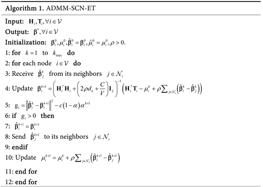Node i continuously observes the state of output weights ${\beta }_i\left(k\right)$ to detect whether the event trigger condition ${\text{g}}_i\left(k\mathrm{,}{e}_i^k\right)>0$ is satisfied. This event-triggered communication algorithm based on ADMM is named ADMM-SCN-ET. The algorithm is shown in Algorithm 1.

4. Numerical Verification

It is easy to understand that if the trigger function part is removed, that is, only the algorithm (22) is used, ADMM-SCN-ET will become a new algorithm ADMM-SCN. In this section, we will compare these two algorithms to prove that the newly proposed distributed improved algorithm can effectively reduce the amount of communication between network nodes.

4.1. Regression on Conhull Dataset

The data set is obtained from the real-valued function given by the following formula [16]:

$f\left(x\right)=0.2{\text{e}}^{-{\left(10x-4\right)}^2}+0.5{\text{e}}^{-{\left(80x-40\right)}^2}+0.3{\text{e}}^{-{\left(80x-20\right)}^2}.$ (31)

We set the sample size of the dataset to 600, randomly selected in $\left[\mathrm{0,1}\right]$, which is a uniform distribution. Similarly, a test dataset with a sample size of 600 is randomly generated in the range of $\left[\mathrm{0,1}\right]$.

In the simulation experiment using dataset Conhull, the network topology of node $V=4$ is shown in Figure 1(a). The regression fitting results of the test dataset using the algorithms ADMM-SCN-ET and ADMM-SCN are shown in Figure 1(b), where the parameter is $L=400,\rho =0.1,k=200$. In addition, the trigger parameter related to the event-triggered communication mechanism set by the algorithm ADMM-SCN-ET is $c=2^2\mathrm{,}\alpha ={\text{e}}^{-0.04}$. By carefully observing the fitting effect of the peak data, we can see that the fitting result using ADMM-SCN-ET is slightly better than that using ADMM-SCN. This situation shows that the proposed event-triggered communication mechanism algorithm ensures the performance of the existing distributed learning algorithm. Figure 1(c) shows the root mean squared error (RMSE) value of regression output, which is used to measure the error between the predicted value and actual value. It can be seen from the figure that RMSE shows a trend of sharp decline first and

(a) (b) (c)

Figure 1. Results of regression on Conhull dataset. (a) Communication network of four agents; (b) Test outputs of the ADMM-SCN-ET and ADMM-SCN; (c) RMSE of the ADMM-SCN-ET.

then slowly increasing and then slowly decreasing again with the final value RMSE = 0.008. And the RMSE of the ADMM-SCN algorithm with the same parameters is 0.017.

The trajectories of nodes ${\Vert e_i\left(k\right)\Vert }^2={\Vert {\beta }_i\left(k\right)-{\hat{\beta }}_i\left(k\right)\Vert }^2$ and $c\left(1-\alpha \right){\alpha }^k$ in the ADMM-SCN-ET algorithm are shown in Figure 2, in which the parameters are $c=2^4\mathrm{,}\alpha ={\text{e}}^{-0.05}$. When the red line value becomes zero, it means that the node has carried out information communication. Figure 3 shows the communication time of each node. Figure 3(a) shows that all node events occur in the case of time trigger, that is, information communication is carried out between nodes in each iteration, Figure 3(b) shows the node communication time in the case of event trigger when parameters are $c=2^2\mathrm{,}\alpha ={\text{e}}^{-0.04}$, the communication times of the four nodes are: 42 times for node 1, 40 times for node 2, 44 times for node 3 and 44 times for node 4. The calculation shows that the total communication times of ADMM-SCN-ET algorithm in this example is 21.21% of ADMM-SCN algorithm in the same communication network topology, saving 78.75% of communication resources.

4.2. Classification on 2Moons Dataset

The 2Moons dataset is an artificial dataset where the data points are divided into two clusters with distinct moon shapes [10]. The global training dataset is 300 points randomly selected from the uniform distribution $\left[-\mathrm{10,10}\right]$. The sample

Figure 2. Trajectories of ${\Vert e_i\left(k\right)\Vert }^2={\Vert {\beta }_i\left(k\right)-{\hat{\beta }}_i\left(k\right)\Vert }^2$ and $c\left(1-\alpha \right){\alpha }^k$ for each node.

(a)(b)

Figure 3. The communication time of eachagent. (a) In the case of time trigger, all nodes communicate every iteration; (b) In the case of event trigger, all nodes communicate when the trigger conditions are met.

size of the test dataset is 100, which is extracted from the regular spacing grid on $\left[-\mathrm{0.5,1.5}\right]$. The numerical simulation results are shown in the following figures.

The network diagram used in this data classification example is shown in Figure 4(a), where node $V=10$. Figure 4(b) shows the classification result of 2Moons dataset when the parameter is $L=\mathrm{500,}\rho =\mathrm{0.1,}k=\mathrm{100,}c=2^2\mathrm{,}\alpha ={\text{e}}^{-0.031}$. In the figure, circles are used to represent the training points of class 1, squares are used to represent the training points of class 2, and the classification boundaries are colored with blue and orange respectively. Figure 4(c) shows the confusion matrix of test dataset classification using the algorithm ADMM-SCN-ET. From the confusion matrix, it can be seen that the classification results of the algorithm are all correct, which proves that the distributed learning algorithm has a strong learning ability for data classification. Figure 4(d) shows the accuracy and RMSE output of ADMM-SCN-ET for classification training. The figure shows that when the hidden layer node of the neural network is greater than 50, the classification accuracy of the training is kept at 1, and RMSR continues to drop to the minimum, with the final value RMSE = 0.021. Under the same parameters, the RMSE of the ADMM-SCN algorithm is 0.017, which ensures the accuracy of the distributed learning algorithm.

The communication time of each node in this example is shown in Figure 5. Figure 5(a) shows the time trigger situation, and all node events occur, Figure 5(b) shows the event trigger situation, and the communication times of each node are: 18 times for node 1, 19 times for node 2, 20 times for node 3, 19 times

(a) (b) (c) (d)

Figure 4. Results of classification on 2Moons dataset. (a) Communication network of ten agents; (b) Test output of the ADMM-SCN-ET; (c) Confusion matrix of the ADMM-SCN-ET; (d) RMSE of the ADMM-SCN-ET.

for node 4, 20 times for node 5, 19 times for node 6, 20 times for node 7, 22 times for node 8, 18 times for node 9, and 19 times for node 10. The total communication times trained by ADMM-SCN-ET algorithm is 19.4% of that trained by the ADMM-SCN algorithm under the same communication network topology, which saves 80.6% of communication resources.

4.3. Classification on MNIST Dataset

The MNIST dataset is a handwritten dataset initiated and organized by the National Institute of Standards and Technology. A total of 250 different person’s handwritten digital pictures are counted, 50% of which are high school students and 50% are from the staff of the Census Bureau. The dataset includes two parts:

(a)(b)

Figure 5. The communication time of each node. (a) In the case of time trigger, all nodes communicate every iteration; (b) In the case of event trigger, all nodes communicate when the trigger conditions are met.

60,000 training datasets and 10,000 test datasets. Each data unit includes a picture containing handwritten digits and a corresponding label. Each picture contains 28 × 28 pixels, and the corresponding label ranges from 0 to 9 representing handwritten digits from 0 to 9. As shown in Figure 6(a).

The network diagram used in this data classification example is shown in Figure 6(b), where node $V=10$. Figure 6(c) shows the confusion matrix of test dataset classification using the algorithm ADMM-SCN-ET when the parameter is $L=1500,\rho =0.1,k=100,c=0.15,\alpha ={\text{e}}^{-0.04}$. The numbers 1 - 10 in the confusion matrix represent the handwritten numbers 0 - 9, respectively. From the results, it can be seen that the classification accuracy of the ADMM-SCN-ET algorithm test set is finally 89.6%. Figure 6(d) shows the accuracy and RMSE output of ADMM-SCN-ET for classification training. This figure shows that as the hidden layer nodes of the neural network gradually increase, the classification accuracy of the final training reaches 89.6%. Under the same parameters, the classification accuracy of the final training of the algorithm ADMM-SCN is 89.5%, and the RMSE value continues to decrease to the lowest point 0.546, the final RMSE value obtained by the ADMM-SCN algorithm of full communication under the same parameters is 0.548, which guarantees the accuracy of the distributed learning algorithm.

The communication time of each node in this example is shown in Figure 7. Figure 7(a) is the time-driven situation, all node events occur; Figure 7(b) is the communication moment when the event-driven communication mechanism is

(a) (b) (c) (d)

Figure 6. Results of classification on MNIST dataset. (a) Examples of the MNIST dataset; (b) Communication network of ten agents; (c) Confusion matrix of the ADMM-SCN-ET; (d) RMSE of the ADMM-SCN-ET.

used, the communication times of each node are: node 1 is 10 times, node 2 is 8 times, node 3 is 6 times, node 4 is 9 times, node 5 is 10 times, node 6 is 10 times, node 7 is 10 times, node 8 is 9 times, node 9 is 10 times, and node 10 is 10 times. The calculation can be obtained when the parameter is $k=100,c=0.15$ and $\alpha ={\text{e}}^{-0.04}$. The total communication times trained by ADMM-SCN-ET algorithm is 9.2% of that trained by ADMM-SCN algorithm under the same communication network topology, which saves 90.8% of communication resources.

Therefore, the simulation results of these three examples show that the proposed distributed learning algorithm can effectively reduce the traffic of distributed learning algorithms in data regression and classification while ensuring the performance of existing distributed learning algorithms.

(a)(b)

Figure 7. The communication time of each node. (a) In the case of time trigger, all nodes communicate every iteration; (b) In the case of event trigger, all nodes communicate when the trigger conditions are met.

5. Conclusion

This paper designs a distributed algorithm based on an event-triggered communication mechanism called ADMM-SCN-ET. Combined with the ADMM for solving the convex consensus optimization problem, we propose a communication-censored distributed learning algorithm and use it to solve the optimal output weight problem of neural networks. The algorithm uses an event-triggered communication mechanism to prevent the transmission of variable information with a small change of node state, and reduces unnecessary information communication between nodes. Finally, three datasets are used to verify the effectiveness of the proposed algorithm. The simulation results show that the algorithm proposed in this paper can effectively reduce the communication traffic of distributed learning algorithms while ensuring the performance of existing distributed learning algorithms in data regression and classification.

Acknowledgements

This work was supported in part by the National Natural Science Foundation of China (No. 62166013), the Natural Science Foundation of Guangxi (No. 2022GXNSFAA035499) and the Foundation of Guilin University of Technology (No. GLUTQD2007029).

Conflicts of Interest

The authors declare no conflicts of interest.

References

[1]	Bekkerman, R., Bilenko, M. and Langford, J. (2011) Scaling Up Machine Learning: Parallel and Distributed Approaches. Cambridge University Press, Cambridge. https://doi.org/10.1145/2107736.2107740
[2]	Bi, X., Zhao, X., Wang, G., Zhang, P. and Wang, C. (2015) Distributed Extreme Learning Machine with Kernels Based on Mapreduce. Neurocomputing, 149, 456-463. https://doi.org/10.1016/j.neucom.2014.01.070
[3]	Georgopoulos, L. and Hasler, M. (2014) Distributed Machine Learning in Networks by Consensus. Neurocomputing, 124, 2-12. https://doi.org/10.1016/j.neucom.2012.12.055
[4]	Brandolese, A., Brun, A. and Portioli-Staudacher, A. (2000) A Multi-Agent Approach for the Capacity Allocation Problem. International Journal of Production Economics, 66, 269-285. https://doi.org/10.1016/S0925-5273(00)00004-9
[5]	Scardapane, S. and Di Lorenzo, P. (2017) A Framework for Parallel and Distributed Training of Neural Networks. Neural Networks, 91, 42-54. https://doi.org/10.1016/j.neunet.2017.04.004
[6]	Shnayder, V., Hempstead, M., Chen, B.R., Werner-Allen, G. and Welsh, M. (2004) Simulating the Power Consumption of Large-Scale Sensor Network Applications. Proceedings of the 2nd International Conference on Embedded Networked Sensor Systems, Baltimore, 3-5 November 2004, 188-200. https://doi.org/10.1145/1031495.1031518
[7]	Heemels, W.P., Johansson, K.H. and Tabuada, P. (2012) An Introduction to Event-Triggered and Self-Triggered Control. 2012 IEEE 51st Conference on Decision and Control (CDC), Maui, 10-13 December 2012, 3270-3285. https://doi.org/10.1109/CDC.2012.6425820
[8]	Liu, Q., Wang, Z., He, X. and Zhou, D. (2014) A Survey of Event-Based Strategies on Control and Estimation. Systems Science & Control Engineering: An Open Access Journal, 2, 90-97. https://doi.org/10.1080/21642583.2014.880387
[9]	Nowzari, C., Garcia, E. and Cortés, J. (2019) Event-Triggered Communication and Control of Networked Systems for Multi-Agent Consensus. Automatica, 105, 1-27. https://doi.org/10.1016/j.automatica.2019.03.009
[10]	Yang, J., Xiao, F. and Ma, J. (2018) Model-Based Edge-Event-Triggered Containment Control under Directed Topologies. IEEE Transactions on Cybernetics, 49, 2556-2567. https://doi.org/10.1109/TCYB.2018.2828645
[11]	Ge, X., Han, Q.L., Ding, L., Wang, Y.L. and Zhang, X.M. (2020) Dynamic Event-Triggered Distributed Coordination Control and Its Applications: A Survey of Trends and Techniques. IEEE Transactions on Systems, Man, and Cybernetics: Systems, 50, 3112-3125. https://doi.org/10.1109/TSMC.2020.3010825
[12]	Dimarogonas, D.V. and Johansson, K.H. (2009) Event-Triggered Control for Multi-Agent Systems. Proceedings of the 48h IEEE Conference on Decision and Control (CDC) Held Jointly with 2009 28th Chinese Control Conference, Shanghai, 15-18 December 2009, 7131-7136. https://doi.org/10.1109/CDC.2009.5399776
[13]	Dimarogonas, D.V., Frazzoli, E. and Johansson, K.H. (2011) Distributed Event-Triggered Control for Multi-Agent Systems. IEEE Transactions on Automatic Control, 57, 1291-1297. https://doi.org/10.1109/TAC.2011.2174666
[14]	Wang, D. and Li, M. (2017) Stochastic Configuration Networks: Fundamentals and Algorithms. IEEE Transactions on Cybernetics, 47, 3466-3479. https://doi.org/10.1109/TCYB.2017.2734043
[15]	Bazaraa, M.S. and Goode, J.J. (1973) On Symmetric Duality in Nonlinear Programming. Operations Research, 21, 1-9. https://doi.org/10.1287/opre.21.1.1
[16]	Tyukin, I.Y. and Prokhorov, D.V. (2009) Feasibility of Random Basis Function Approximators for Modeling and Control. 2009 IEEE Control Applications, (CCA) & Intelligent Control, (ISIC), St. Petersburg, 8-10 July 2009, 1391-1396. https://doi.org/10.1109/CCA.2009.5281061