On Fermat’s Last Theorem and Galaxies of Sequences of Positive Integers ()
Cubum autem in duos cubos, aut quadratoquadratum in duos quadratoquadratos, et generaliter nullam in infinitum ultra quadratum potestatum in duos ejusdem nominis fas est dividere: Cujes rei demonstrationem mirabilem sane detexi. Hane marginis exiguitas non caperet.—Pierre de Fermat (1637)
1. Introduction and Main Result
It is well that there are many solutions in positive integers to the equation
, for instance (3, 4, 5); (5, 12, 13). Around 1500 B.C., the Babylonians were aware of the solution (4961, 6480, 8161) and the Egyptians knew the solutions (148, 2736, 2740) and (514, 66,048, 66,050). Also Greek mathematicians were attracted to the solutions of this equation. We notice that this equation has sequences of complex number solutions
(1.1)
and matrix solutions
(1.2)
In 1637, Pierre de Fermat wrote a note in the margin of his copy of Diophantus Arithmetica [1] stating that the equation
(1.3)
has no positive integer solutions. This is the Fermat Last Theorem. He claimed that he had found the proof of this Theorem. The only case Fermat actually wrote down a proof is the case
. In his proof, Fermat introduced the idea of infinite descent which is the main tool in the study of Diophantine equations. He proved that the equation
has no solutions in relatively prime integers with
. Solutions to this equation correspond to rational points on the elliptic curve
. The proof of the case
was given first by Karl Gauss. In 1753, Leonhard Euler gave a different prove of Fermat’s Last Theorem for
[2] [3]. In 1823, Sophie Germain proved that if l is a prime and 2l + 1 is also prime, the equation
has no solutions (x, y, z) with
. The case
was proved simultaneously by Adrien Marie Legendre in 1825 [4] [5] and Peter Lejeune Dirichlet [6] in 1832. In 1839, Gabriel Lame proved the case
[7] [8] [9] [10]. Between 1840-1843, V. A. Lebesque worked on Fermat’s Last Theorem [11] [12]. Between 1847 and 1853, Ernst Eduard Kummer published some masterful papers about this Theorem. Fermat’s Last Theorem attracted the attention of many researchers and many studies have been developed around this Theorem. For example the work of Arthur Wieferich (1909), Andre Weil (1940), John Tate (1950), Gerhard Frey (1986), who was the first to suggest that the existence of a solution of the Fermat equation might contradict the modality conjecture of Taniyama, Shimura and Weil [13]; Jean Pierre Serre (1985-1986) [14] [15] [16], who gave an interested formulation and (with J. F. Mestre) tested numerically a precise conjecture about modular forms and Galois representations mod p and proved how a small piece of this conjecture the so called epsilon conjecture together Modularity Conjecture would imply Fermat’s Last Theorem; Kennedy Ribet (1986) [17], who proved Serre’s epsilon conjecture, thus reducing the proof of Fermat’s Last Theorem; Barry Mazur (1986), who introduced a significant piece of work on the deformation of Galois representations [18] [19]. However, no final proof was given to this Theorem. This Theorem was unsolved for nearly 350 years. In 1995, using Mazur’s deformation theory of Galois representations, recent results on Serre’s conjecture on the modularity of Galois representations, and deep arithmetical properties of Hecke algebras, Andrew Wiles with Richard Taylor succeeded in proving that all semi-stable elliptic curves defined over the rational numbers are modular. This result is less than the full Shimura-Taniyama conjecture. This result does imply that the elliptic curve given above is modular. Therefore, proving Fermat’s Last Theorem [20] [21]. Many mathematicians are still heavenly involved on studying Fermat’s Last Theorem [22] [23] [24]. In 2021, Nag introduced an elementary proof of Fermat’s Last Theorem for epsilons [25].
This Theorem has many applications in Cryptography.
It is well known that Fermat’s Last Theorem is true. Now we know that only the equation
admits positive integer solutions. Perhaps it will be a good idea of investigating the properties of these solutions and found out the applications of these solutions. For more than 3500 years, no sequences of triples of positive integers solutions of this equation were introduced before. This paper is structured as follows. In Section 2, we show that the universe
is not empty. In Section 3, we introduce Mouanda’s choice functions which allow us to construct in Section 4, Section 5 and section 6, practical examples of galaxies of triples of positive integers solutions of the equation
. In Section 7, we give the characterization of these solutions. This characterization allows us to prove our main result.
Theorem 1.1. The equation
(1.4)
has no positive integer solutions.
We also prove that the equation
has no positive integer solutions. Our study generates problems which are still unsolved. Since the creation, humans had a big strangle to understand the universe. This strangle did lead to the invention of telescopes. This instrument did allow humans to have clear pictures of galaxies of the universe. It becomes so crucial to create other tools which could lead to a better understanding of the structure and laws of the universe. Perhaps a mathematical tool will be cheaper. In Section 8, we introduce the main reasons why the Fermat Last Theorem is true. In Section 9, we show that every multiverse of triples of complex numbers contains a finite number of universes. This result was predicted in 2018 by Stephen Hawking [26]. We also identify every triple
of
as the continuous function
defined by
The graph of the function
is the sphere of centre
. In Section 10, we introduce the planetary representation of the complex universe
links to sequences of triples of complex numbers which satisfy the equation
. This equation is considered as the stability law of the complex universe
. This planetary representation is the mathematical tool which allows us to have a clear understanding of the structure and laws of the universe. This mathematical tool allows us to predict the structure, laws of the universe. In Section 11, we predict life in every planet system of every galaxy of the universe.
2. Triples of Positive Integers Solutions of the Equation
In this section, we construct sequences of triples of positive integers which are solutions of the equation
. The characterization of these solutions allows us to deduce that the equation
has no solutions in
.
Let
be three positive integers such that
. There exist two positive integers
such that
and
. The equation
(2.1)
is reduced to
(2.2)
It follows that
(2.3)
This implies that
(2.4)
Define the complex polynomial
by setting
(2.5)
Remark 2.1 The roots of the polynomial
(2.6)
are solutions of the equation
(2.7)
Definition 2.2. Let
be complex numbers. Denote by
(2.8)
The triple
is called the triple
to the power n.
Definition 2.3. Let
be complex numbers. Denote by
(2.9)
Definition 2.4. A universe of degree
of the algebra
is the set
of triples
of elements of
which satisfy the law of stability
The element
is called a star (or a planet)of the universe
.Every sequence
of elements of the universe
is called a planet system of elements of
.
The set
is called the complex universe of degree
. In particular, the set
is called the natural universe of degree n. It well known that the natural universe
is not empty. Fermat’s Last Theorem is equivalent to say that
In other words, there are complex universes which don’t have triples of positive integers as elements. We can show that the natural universe
is not empty.
Theorem 2.5. There exist an infinite number of sequences of triples of positive integers
such that
Proof. Let
be three positive integers such that
. Then there exist two positive integers
such
(2.10)
It follows that
(2.11)
This implies that
(2.12)
It is well known that
(2.13)
and
(2.14)
The Equation (2.12) is reduced to
(2.15)
Define the complex polynomial
by setting
Let us calculate the roots of the polynomial
in
. We have the following
(2.16)
There are two solutions which are
(2.17)
and
(2.18)
It is straightforward to see that the roots
of the polynomial
depend on
and
. For example, the possible values of
and
which can probably make
(or
) a positive (or negative) integer are
(2.19)
In this case,
. Therefore,
(2.20)
and
(2.21)
Finally, if we assume that
, then
are roots of the polynomial
. Define the sequence of triples
by setting
(2.22)
(2.23)
and
(2.24)
A simple calculation shows that
(2.25)
and
(2.26)
There are several ways of constructing sequences
of triples of positive integers which satisfy the Equation (2.25). For example, if we choose
and
, then
(2.27)
and
(2.28)
Now, with
we can construct a new sequence of triples
by setting
(2.29)
(2.30)
and
(2.31)
A simple calculation shows that
(2.32)
and
(2.33)
● Actually, there exists an infinite number of ways of choosing
and
. For example, let us choose
and
. In this case,
(2.34)
and
(2.35)
Therefore, the sequence of triples
defined by setting
(2.36)
(2.37)
and
(2.38)
satisfy
(2.39)
and
(2.40)
● Once again, let now choose
and
. We can compute
(2.41)
(2.42)
and
(2.43)
Again, we have the following:
(2.44)
and
(2.45)
A simple observation of the construction of the triple
allows us to set up our first model of sequences of triples of positive integers which satisfy the Equation (2.5). Assume that
(2.46)
(2.47)
and
(2.48)
The elements of the sequence of triples
satisfy
(2.49)
and
(2.50)
Perhaps it is possible to construct another model of sequences of triples of positive integers which depends on two parameters. Let us choose
and
with
(2.51)
We can compute
(2.52)
(2.53)
and
(2.54)
The triples
satisfy
(2.55)
and
(2.56)
The construction of this sequence of triples allows us to set up our second model of sequences which satisfy the Equation (2.55). Let us replace 3 in
by a. In other words,
(2.57)
(2.58)
and
(2.59)
The elements of the sequence of triples
satisfy
(2.60)
and
(2.61)
We can now claim that the natural universe
has no power element.
3. Mouanda’s Choice Functions
Denote by
, the set of complex functions over
. Let
be the set of all subsets of
. Theorem 2.5 allows us to claim that the appropriate choice of the values of
and
such that
(3.1)
leads to the construction of sequences of triples of positive (or negative) integers which satisfy the equation
(3.2)
Let
be the function defined by
let
be the function defined by
let
be the function defined by
let
be the function defined by
let
be the function defined by
let
be the function defined by
let
be the function defined by
and let
be the function defined by
These type of functions are called Mouanda’s choice functions. Mouanda’s choice functions are galaxy valued functions. These functions allow us to construct galaxies of numbers or matrices.
4. The Model of the Galaxy of Galaxies of Sequences of Positive Integers of order 1
Definition 4.1. The order of a galaxy is the number of variables of the galaxy.
Mouanda’s choice function
allows us to construct galaxies of numbers. For instance, the model
is called the galaxy of sequences of positive integers of order 2, base
. For
and a fixed, the triple
is called the origin of the galaxy
. The elements of
satisfy
(4.1)
and
(4.2)
Example 4.2. Galaxies of Sequences of Positive Integers with Square Bases of order 2
● The model
is called the galaxy of sequences of positive integers of order 1. The triple
is called the origin of the galaxy
. The triple
satisfies
(4.3)
(4.4)
and
(4.5)
● The model
is called the galaxy of sequences of positive integers of order 0. Every sequence can be identified as a galaxy of order 0. We have
(4.6)
and
(4.7)
● The elements of the sequence
satisfy
(4.8)
and
(4.9)
● The elements of the galaxy
satisfy
(4.10)
and
(4.11)
● The elements of the galaxy
satisfy
(4.12)
and
(4.13)
Example 4.3. Different Models of Galaxies with no Square Bases
The triples
of the galaxy
satisfy
(4.14)
(4.15)
and
(4.16)
Example 4.4. The triples
of the galaxy
satisfy
(4.17)
and
(4.18)
Example 4.5. The triples
of the galaxy
satisfy
(4.19)
and
(4.20)
Example 4.6. The triples
of the galaxy
satisfy
(4.21)
and
(4.22)
5. Σ-Model
The triples
of the galaxy
satisfy
(5.1)
(5.2)
and
(5.3)
Example 5.1. The triples
of the galaxy
satisfy
(5.4)
(5.5)
and
(5.6)
Example 5.2. The triples
of the galaxy
satisfy
(5.7)
(5.8)
and
(5.9)
6. Power Models of Galaxies of Sequences of Positive Integers of Order 3
A model of a galaxy is a power model if the power of the lead of the model is a power. For example, if we choose
and
, the model
is a power model. The elements of the model
satisfy
(6.1)
and
(6.2)
Example 6.1. The elements of the galaxy
satisfy
(6.3)
and
(6.4)
Example 6.2. If we choose
and
, we could construct the galaxy
The elements of this galaxy satisfy
(6.5)
and
(6.6)
The model
is called the galaxy of sequences of positive integers of order 1. The model
is called the galaxy of galaxies of sequences of positive integers of order 2. The model
is called the galaxy of galaxies of sequences of positive integers of order 3.
7. Construction of the Galaxy of Sequences of Positive Integers of Order 4 and Proof of the Main Result
In this section, we prove our main result and we show that there are galaxies which are bigger than the galaxy
. Recall that
Let us choose
as a function of two variables in
. One has the GADA model defined by
The elements of the galaxy
satisfy
(7.1)
The order of the galaxy
is 4.
Example 7.1. The elements of the galaxy
satisfy
(7.2)
We can now give the characterization of the solutions of the equation
.
Remark 7.2. Let
be positive integers such that
(7.3)
Then
(7.4)
(7.5)
and
(7.6)
Theorem 2.5 and Remark 7.2 allow us to prove our main result.
Proof of Theorem 1.1.
Assume that there exist three positive integers
such that
(7.7)
This means that
(7.8)
Therefore,
(7.9)
We have a contradiction because the set
has no power element. Finally, there exist no positive integers
such that
(7.10)
Our main result allows us to claim that there exist no positive integers
such that
(7.11)
Our main result allows us to prove Fermat’s Last Theorem for
.
Theorem 7.3. Let
be an element of the complex universe
(7.12)
Then
.
Proof. Let
. Then
(7.13)
This implies that
(7.14)
and
(7.15)
We can now claim that the elements of the universe
have the same properties. Theorem 1.1, Theorem 2.5 and Remark 7.2 allow us to claim that
(7.16)
since
has no power solutions. In other words,
(7.17)
The fact that
(7.18)
implies that
(7.19)
8. The Main Reasons Why Fermat’s Last Theorem Is True
The main reasons why the Fermat Last Theorem is true are:
●
, one has
(8.1)
●
, one has
(8.2)
● Every element
satisfies
(8.3)
● Every element
satisfies
(8.4)
8.1. Problems
Our study generates several problems:
Problem 1: How can we construct the galaxy of galaxies of sequences
.
Problem 2: How can we construct other models of the galaxies of sequences links to the root
Problem 3: How can we construct models of galaxies of sequences of real numbers generated by the roots of the polynomial
defined by setting
Problem 4: How can we construct models of the galaxy of galaxies of sequences of real numbers generated by the roots of the polynomial
defined by setting
The resolution of these problems will lead to the birth of a new theory called Galaxies of Numbers Theory.
8.2. What We Learn
We learn so far that the equation
is the law of stability of the universe of sequences of positive integers. Also, the distance between the origin of the galaxy Gala(9, a), which is
and the second element of the sequence
of the galaxy
, which is
is fixed. We can claim that origins of galaxies are connected to sequences of other galaxies. It follows that all the sequences of the universe of sequences of positive integers which satisfy the equation
are linked to each other and are in parfait harmony by the law of stability.
9. Disjoint Multiverses of Complex Numbers
A multiverse (or parallel universes) is the collection of alternate universes that share a universal hierarchy. The idea of the existence of the multiverse has been around for long time. An idea which many theoretical physicists have been trying to prove by using string theory which is a branch of theoretical physics that attempts to reconcile gravity and general relativity with quantum physics. In 2018, Stephen Hawking on his paper entitled “A smooth exit from eternal inflation?” predicted that there are not infinite parallel universes in the multiverse, but instead a limited number and these universes would have laws of physics like our own [26]. Perhaps our strangle of understanding the existence of the multiverse and its structure is coming from the absence of a strong mathematical tool capable of representing our entire universe in terms of triples of numbers. Representation theory and continuous functions would play an important role here. Our mathematical approach of describing the structure of a multiverse allows us to observe that disjoint multiverses are made of finite number of universes which have different stability laws. It is quiet clear that our observation is exactly the same to the one predicted in 2018 by Stephen Hawking. In this section, we are going to show that it is possible to associate triples
of complex numbers which satisfy the equation
with planet systems of a universe. Our representation allows us to show that every planet (or star) can be associated to the graph of an appropriate continuous function which depends on the triple
of complex numbers of a universe and our universe is made of an infinite number of galaxies.
9.1. nth Root of a Complex Number
It is well known that de Moivre’s formula can be used to compute roots of complex numbers. Assume that n is a positive integer and
is the nth root of the complex number z denoted by
, then we have
. Let
(9.1)
and
(9.2)
Due to the fact that
, we can claim that
(9.3)
The well known de Moivre Theorem allows us to say that
(9.4)
It follows that
(9.5)
The distinct values of the nth root of the complex number
are
(9.6)
In other words,
(9.7)
We can deduce the solutions of the equation
which are:
(9.8)
This means that the equation
, would have the set
(9.9)
as the set of solutions. In the same way, we could say that the equation
, would have the complex numbers
(9.10)
as solutions. We know that
. We can construct elements of
. Let us compute
. Assume that
(9.11)
That is,
(9.12)
(9.13)
and
(9.14)
The triples
satisfy the equation
.
9.2. Multiverse (or Parallel Universes) of Complex Numbers
In this section, we show that every multiverse contains a finite number of universes. Mouanda’s choice functions could allow us to compute the complex solutions of the equation
. Denote by
The set
is called the first universe of complex numbers (or complex universe of degree 2). For example, the triples
of complex number of the galaxy
satisfy
(9.15)
is called the galaxy of galaxies of triples of complex numbers. It follows that
(9.16)
We can say that the universe
is a multiverse which contains at least 4 universes. The set
(9.17)
is called the universe of complex numbers (or complex universe) of degree n. The equation
is the stability law of the complex universe
. The elements of the complex universe
allow us to construct disjoint complex universes
. In fact,
(9.18)
Every element
of the set
generates
elements of the set
. Indeed, let
be an element of the set
. Assume that
(9.19)
and
(9.20)
It is straightforward to see that
(9.21)
Let us notice that
(9.22)
We have an infinite number of disjoint complex multiverses with different structures and stability laws. In other words,
(9.23)
Let
be a triple of complex numbers. Define the continuous function
by setting
(9.24)
The graph of the function
is the sphere of centre
. We can see that every triple of complex numbers
can be associated to a continuous function
over
. The shape of the graph of the continuous function
depends on the values of
.
Example 9.1. Let us consider the galaxy
The functions
associated to the triples
of the planet system
with
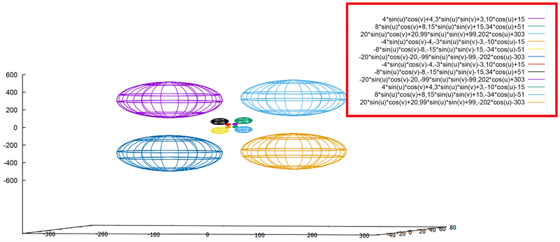
The graphs of
and symmetric functions.
can be represented graphically.A simple calculation shows that
(9.25)
10. The Planetary Representation of
Definition 10.1. The planetary representation of the universe
is the identification process of each triple
of the universe
to the planet
(or the star
) of the associated universe.
In this model of representation, the temperature, the mass, the radius, the orbital period, the surface area, the pressure, the distance between stars (or planets), the speed of rotation and the age limit of a star (or a planet) are functions of
. The investigation of these functions still remains opened. We can now associate every sequence
to a planet system of our universe. The map
defined by
can be considered as the planetary representation of the complex universe
. On this basis, we have the following observations.
Remark 10.2. Prediction of the Structure and Laws of the Universe. The universe:
● Has no centre.
● Has no origin (beginning).
● Has no end.
● Has an infinite number of galaxies.
● The origins of all galaxies are linked by the stability law.
● All the galaxies are linked by the stability law.
● Galaxies of the same base
are on the same plate.
● All the galaxies are generated from one identity structure
,for example,the galaxies of sequences
and
are generated from the roots of the function
.
● To keep his eternal nature,the death of one star is immediately replaced by the birth of another star.The death of one galaxy gives birth to another galaxy.The death of one planet system gives birth to a new planet system.
● Our solar system has undiscovered planets links to other galaxies.
● Due to the fact that the sun has got a destroyable structure in time,our solar system will cease to give birth to another planet system with life on it.
● The sun turn around another planet of our galaxy.
● Every day new planet systems are born.
● The galaxies of the universe are in motion by keeping in them the law of stability.
● Humans are linked to every thing which exists on earth.
All these observations allow us to claim that humans need a clear understanding of their relationships with every thing on earth because their survival depends on it.
11. Prediction of Life in Every Planet System of the Universe
The stability law of the natural universe
allows us to claim that there is life in every planet system of every galaxy.
Theorem 11.1. There is life in every planet system of every galaxy of the universe. In other words, in each planet system of every galaxy of the universe, there exists a planet with life on it.
Proof. Only the natural universe
is not empty at all and the other natural universes
are completely empty. First of all, let us notice that all the sequences of the galaxy of order 1
have the same shape and geometry and all the galaxies of order 1 of the galaxy of order 2
have the same shape. The galaxy
can be considered as a subset of the natural universe
. The planetary representation of the galaxy
allows us to say that each element
of any sequence of the galaxy
can be identified as the star
(or the planet
) of our universe and the temperature, the mass, the radius, the orbital period, the surface area, the pressure, the distance between stars (or planets), the speed of rotation and the age limit of every star (or planet) are functions of
. The stability law and the planetary representation of the natural universe
allow us to claim that every planet system of our galaxy has the same properties. This means that every planet system of our galaxy has got a sun. The fact that our solar system got life on it means that there is life too in every single planet system of our galaxy. The stability law allows us to claim that wherever you see a sun in our universe, that sun is linked to a planet system which got life on it.
12. Conclusions
● Let
(or
) be a star (or planet) of our universe. Then
(12.1)
● On earth:
1)
(12.2)
Therefore, the stability law on earth is love.
2) HATE is the law of self-destruction.
3) Every body came from the same origin.
4) Galaxy of Numbers Theory is linked to Astronomy.