The Light Timing Calculations of the Interferometer in the Quest to Detect Light Speed Anisotropy and a Case Study of the Michelson-Morley and Miller Mt Wilson Experiments

Declan Traill

Melbourne, Australia.

DOI: 10.4236/jamp.2022.103055                

Abstract

This paper formulates the light timing calculations for each interferometer arm; one that is parallel to the direction of motion of the interferometer through space and the other that is perpendicular. The calculations are done for a vacuum-mode interferometer and then for a gas-mode interferometer. The calculations show that no light timing difference is detectable in a vacuum-mode interferometer, but once an optical medium is present in the light path down the arms of the interferometer, this is no longer the case and a timing difference is detectable. Further to this, the timing equations obtained from the analysis are used to model the historical experiments of Michelson-Morley and Miller (Mt Wilson) and predictions are made by the model that accurately match the actual recorded results from those experiments. Thus, this timing analysis confirms that there is a light speed anisotropy in a reference frame that is moving through space, indicating the presence of a preferred Aether reference frame through which the Earth is moving.

Keywords

Interferometer, Luminiferous, Aether, Michelson, Morley, Miller, Wilson, Light, Interference, Fringe, Timing, Isotropic, Anisotropic, Preferred, Reference, Frame, NASA, Doppler, Anomaly, Cahill, Computer, Model, Gas, Mode, Vacuum

1. Introduction

The Luminiferous Aether theory of the 19^th Century was widely considered disproven by the apparently Null result of the Michelson-Morley result whose aim was to reveal the Earth’s motion through the Aether. Whilst the results of the experiment were not completely Null, there was a much smaller fringe shift in their interferometer than had been expected, so the conclusion was drawn that if there was an Aether, Earth’s motion through it was negligible.

In 1887, Michelson and Morley [1] described that “It appears, from all that precedes, reasonably certain that if there be any relative motion between the earth and the luminiferous ether, it must be small; quite small enough entirely to refute Fresnel’s explanation of aberration. Stokes has given a theory of aberration which assumes the ether at the earth’s surface to be at rest with regard to the latter.” The conclusion was “the ether is at rest with regard to the earth’s surface.”

Further tests were done by several people, including Miller [2] who conducted his experiment at the top of Mt Wilson in an attempt to remove the interferometer from any entrained Aether effect associated with being close to the Earth’s surface. He obtained similar results, although in his case the result was more conclusively not Null, but still small.

Miller’s conclusion, after conducting about 5000 single measures of the Aether drift over a period of four years was that [3] “there is a positive displacement of the interference fringes, such as would be produced by a relative motion of the earth and the ether at this Observatory.” So, clearly, Miller was of the opinion that the Earth is in motion relative to the Aether and my experimental work and mathematical Physics modelling agree with this assessment, yet he went on to say that “…of approximately ten kilometres per second, being about one-third of the orbital velocity of the earth.”

I disagree with this part of the assessment as this conclusion has been drawn based on incorrect mathematical modelling of the situation of the interferometer experiment. In this paper, I demonstrate and explain the correct mathematical modelling for this type of experiment and show that this modelling predicts the same magnitude of interference fringe shift as was measured and recorded by both Michelson-Morley and Miller in their respective experimental results.

Subsequent to these experiments, Lorentz proposed the Lorentz-Fitzgerald Length Contraction effect (a part of the Lorentz transformations, which became a key part of Einstein’s Relativity theory) which indicated that the length of any object in motion would be contracted due to that motion. It just so happens that (in a vacuum at least) the amount of the length contraction exactly compensates for any timing difference down the orthogonal arms of an interferometer due to the anisotropy in the speed of light that might exist in a moving reference frame, thus making detection of the anisotropy (and thus the motion through the Aether) impossible [4]. Therefore, it seemed impossible to detect any light speed anisotropy and speed through the Aether by using an interferometer.

However, if an optical medium is introduced into the interferometer light paths along its arms (such as the air medium used in the Michelson-Morley and Miller experiments) the calculation becomes more complex, as the air slightly slows the speed of light along its travel path. The effect of the air is not simply that light can be treated at now traveling at c/n (where n is the refractive index of the air) though, as the Fresnel Dragging effect (tested in the Fizeau experiment) proved. The actual effect of the air is to cause the light to be momentarily delayed by each air molecule it encounters, but it still travels at the full speed of light in the vacuum between air molecules. See this paper [5] for a full analysis of how this effect occurs and results in the Fresnel Dragging equation.

To this day there has not been a satisfactory explanation for the Michelson-Morley or Miller experimental results (or any other gas-mode interferometer experiment for that matter) and many simply dismiss their results as experimental error. This paper demonstrates how the interferometer light timings should be calculated to correctly account for the delaying effect of the air molecules. In doing so, it can accurately model the observed results of both the Michelson-Morley and Miller experiments. There also exists other corroborating evidence of the Earth’s motion through the Aether, such as the NASA spacecraft Earth fly-by Doppler measurements and other experiments using coaxial cables to reveal the light speed anisotropy that exists in the Earth’s reference frame [6] [7]. The accurate NASA measurements indicate a speed of the Earth through the Aether of ~486 km/s, so using this Aether wind speed in the model for the Michelson-Morley and Miller experiments I am able to obtain predicted interference fringe shifts for these two experiments of 0.017 and 0.086. These values are in excellent agreement with the recorded measurements from these two experiments [8].

2. The Vacuum-Mode Interferometer

Consider this interferometer setup.

2.1. Part A

A pulse of laser light (depicted as the dashed arrow) is sent across the reference frame (from a source connected to the reference frame) perpendicular to the direction of motion through the Aether field. In the stationary frame, the path length taken by the light is L as expected (Figure 1); but in the moving frame, the path taken is longer (L₁) due to the constant flow of the Aether field through the frame, and the fact that the light moves with a certain velocity with respect to the field, rather than the moving reference frame (Figure 2).

A moving laser will emit a beam that follows the angled path given by L₁—this can be demonstrated with a Huygens construction of the wavelets comprising the beam as it is being emitted, and follows the same principle as the operation of a phased-array radar, where the beam direction can be changed by slightly altering the emission timing of an array of dipole antennas, without physically moving the array.

Light always travels at speed c relative to space (the Aether field), thus:

Figure 1. Light traversing a stationary reference frame, vertically.

Figure 2. Light traversing a reference frame vertically, that is moving from right to left at speed v.

$\Delta t_0=\frac{L}{c}$ (1)

$\Delta t=\frac{L_1}{c}$ (2)

${\left(L_1\right)}^2=L^2+{\left(v\Delta t\right)}^2$ (3)

Using (1) and (3) we have

$L_1=\sqrt{{\left(c\Delta t_0\right)}^2+{\left(v\Delta t\right)}^2}$ (4)

Using (2) gives:

${\left(c\Delta t\right)}^2={\left(c\Delta t_0\right)}^2+{\left(v\Delta t\right)}^2$ (5)

Solving for $\Delta t$ gives

$\Delta t=\frac{\Delta t_0}{\sqrt{1-{\left(\frac{v}{c}\right)}^2}}$ (6)

The Lorentz factor:

$\gamma =\frac{\Delta t}{\Delta t_0}=\frac{1}{\sqrt{1-{\left(\frac{v}{c}\right)}^2}}$ (7)

Equation (7) is the accepted (and verified) equation for calculating the time dilation due to relative motion.

2.2. Part B

Now consider the same situation as depicted in Part A, but with a light pulse sent across the reference frame parallel to the direction of motion.

Consider the light’s journey both in the direction of travel (Figure 3) and in the opposite direction (Figure 4) as separate cases, then combine the results to give an overall, round-trip result. The reference frame travels different distances in each case as $\Delta t_1>\Delta t_2$ . This means that the lights’ actual travel time is different in each direction, but it can be demonstrated that for a round trip the total time dilation during the trip is the same as it was in (Figure 2)—where the light travelled perpendicular to the direction of motion.

Again, light travels at speed c relative to space (the Aether field), giving:

$\Delta t_{\text{up}}=\frac{\frac{L}{\gamma }+v\Delta t_{\text{up}}}{c}$ (8)

$\Delta t_{\text{down}}=\frac{\frac{L}{\gamma }-v\Delta t_{\text{down}}}{c}$ (9)

Figure 3. Light traversing a reference frame that is moving from right to left at speed v. The light is moving horizontally, in the same direction as the frame’s motion through space.

Figure 4. Light traversing a reference frame that is moving from right to left at speed v. The light is moving horizontally, in the opposite direction to the Frame’s motion through space.

Solving for $\Delta t_{\text{up}}$ and $\Delta t_{\text{down}}$ gives:

$\Delta t_{\text{up}}=\frac{L}{\gamma \left(c-v\right)}$ (10)

$\Delta t_{\text{down}}=\frac{L}{\gamma \left(c+v\right)}$ (11)

The round-trip time is defined as:

$\Delta t_a=\Delta t_{\text{up}}+\Delta t_{\text{down}}$ (12)

If $\Delta t_a$ is the total time taken according to observer A, who is stationary in the Aether field, and $\Delta t_b$ is the total time taken according to observer B in the reference frame travelling at speed v through the field. Observer B will have dilated time, so each observer expects that $\Delta t_a>\Delta t_b$ .

${\gamma }_{\text{parallel}}=\frac{\Delta t_a}{\Delta t_b}$ by definition (13)

According to observer B (using his clock), the time taken by the light pulse in his reference frame is simply:

$\Delta t_b=\frac{2L}{c}$ (14)

For observer A, the calculation for the light pulse’s travel time is a little more complicated, as the upstream & downstream times must be considered separately, and then summed:

Using Equations (10), (11) and (12) gives:

$\Delta t_a=\frac{L\left(c+v\right)+L\left(c-v\right)}{c^2-v^2}=\frac{2cL}{c^2-v^2}$ (15)

Then using (13), (14) and (15) he/she is able to calculate ${\gamma }_{\text{parallel}}$ :

${\gamma }_{\text{parallel}}=\frac{\left(\frac{2cL}{c^2-v^2}\right)}{\left(\frac{2L}{c}\right)}=\frac{c^2}{c^2-v^2}$ (16)

So

${\gamma }_{\text{parallel}}=\frac{1}{\left(\frac{c^2-v^2}{c^2}\right)}=\frac{1}{1-{\left(\frac{v}{c}\right)}^2}={\gamma }^2$ (17)

This finding appears, on the face of it, to indicate that the time taken for the light pulse travelling in a direction parallel to the direction of motion would be longer than the time taken for an equivalent light pulse travelling perpendicular to the direction of motion. In fact, the time dilation in the parallel direction appears to be the square of the time dilation in the perpendicular direction.

This situation was investigated in a famous experiment carried out by Michelson & Morley in 1887 in their attempts to discover the effects of the Earth’s motion through the Luminiferous Aether [1]. The expected result of the experiment was that a different travel time would be detected between the parallel & perpendicular light paths (indicated by a shift in interference fringes when the two beams are recombined).

However, much to the astonishment of the experimenters and the rest of the scientific community, the results of the experiment indicated no (or a much smaller than expected) difference in travel times between the two light paths (within the accuracy of the measurements).

The Lorentz-Fitzgerald contraction was proposed to account for this unexpected result, and this formed part of the theory of Relativity. Special Relativity indicates that the length of an object moving at speed contracts to a shorter length as a direct result of the object’s motion. This proposal has since been verified by experiment. However, at the same time as the problem was solved, the Aether theory was rejected in favour of Einstein’s Relativity.

Fitzgerald showed that when Special Relativity is taken into consideration for solid objects, the forces holding that body together adjust is just such a way to cause the body’s length to contract.

The length is shorter by an amount equal to the Lorentz factor.

$\gamma =\frac{1}{\sqrt{1-{\left(\frac{v}{c}\right)}^2}}$ (18)

So, the length of the moving reference frame in the previous calculation is L_b rather than L, where:

$L_b=\frac{L}{\gamma }$ (19)

$\Delta t_a=\frac{L_b\left(c+v\right)+L_b\left(c-v\right)}{c^2-v^2}=\frac{2c{L}_b}{c^2-v^2}$ (20)

Then using (13), (14), (19) and (20) he/she is able to re-calculate ${\gamma }_{\text{parallel}}$ :

${\gamma }_{\text{parallel}}=\frac{\left(\frac{2c{L}_b}{c^2-v^2}\right)}{\left(\frac{2L}{c}\right)}=\frac{c^2}{\gamma \left(c^2-v^2\right)}$ (21)

As we saw in Equation (17) $\frac{c^2}{c^2-v^2}={\gamma }^2$ so,

${\gamma }_{\text{parallel}}=\frac{{\gamma }^2}{\gamma }$ (22)

Finally, ${\gamma }_{\text{parallel}}=\gamma =\frac{1}{\sqrt{1-{\left(\frac{v}{c}\right)}^2}}$ (the Lorentz factor)

So,

$\Delta t_a=\frac{2\gamma L}{c}$ (23)

Thus, we can see that the times taken for a light pulse to travel in the perpendicular and parallel directions in a vacuum-mode interferometer are equal, despite the motion of the experimental apparatus and the observer through the Aether field. This is the same outcome as predicted by Special Relativity theory.

There exists an asymmetry in the travel times of the light pulses in the “upstream” and “downstream” directions, but due to the nature of the measurement of time intervals—which requires comparisons made with reference to a fixed point (a round trip)—the different times sum to give the same time dilation as one would get for light pulses travelling perpendicular to the direction of motion. Therefore, the different travel times occurring in different directions are not detected.

3. The Gas-Mode Interferometer

Now, consider the following situation, where the same interferometer as was just analysed in the case of the vacuum-mode interferometer, is now in a gaseous environment where the gas is stationary relative to the interferometer and has a constant homogenous refractive index of n.

The introduction of an optical medium with refractive index of n into the interferometer arms affects the parallel arm timing by a simple multiplication of the factor n [9], but for the perpendicular arm direction, this is not the case. Thus, when an optical medium (such as air) is introduced into the interferometer then the parallel and perpendicular light timings are no longer identical.

3.1. The Parallel Arm Timing Calculation

For the interferometer arm that is parallel to the direction of motion of the interferometer through space (the Aether field), the calculation can be done from either the point of view of an observer who is stationary in the space/Aether field, or from the point of view of an observer who is in the interferometer’s reference frame (which is moving at speed v through space). If the timing equations used are correct, then the two different perspectives should give the same timing result (so long as the same time units—dilated or non-dilated time, are used).

From the Aether-centric observer’s point of view, the calculation is done like this:

The time taken for the light signal to cross the distance L in the interferometer arm when it is stationary in the Aether is:

$\Delta t_{\text{stationary}}=\frac{Ln}{c}$ (24)

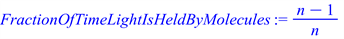
The fraction of the total time that the light is delayed by the air molecules (whilst absorbed and before being re-emitted) is:

${\text{Time Fraction}}_{\text{molecules}}=\frac{n-1}{n}$ (25)

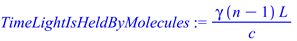
The amount of time that the air molecules delay the light (also from an Aether-centric point of view, hence the γ factor for the Time-Dilation in the moving frame when viewed from the Aether-centric frame) is:

$\Delta t_{\text{molecules}}=\gamma \cdot {\text{Time Fraction}}_{\text{molecules}}\cdot \Delta t_{\text{stationary}}$ (26)

As the air molecules are moving through the Aether whilst the light is absorbed by them, they are either increasing or reducing the optical path length that the light must travel through the Aether during its journey up/down the interferometer arm. So, the up/down optical path length equations become:

$\Delta x_{\text{up}}=\frac{L}{\gamma }+v\Delta t_{\text{up}}-v\Delta t_{\text{molecules}}$ (27)

$\Delta x_{\text{down}}=\frac{L}{\gamma }-v\Delta t_{\text{down}}+v\Delta t_{\text{molecules}}$ (28)

The up/down path timing equations are calculated from the sum of the optical propagation time down these path lengths, plus the time that the light is absorbed by the air molecules:

$\Delta t_{\text{up}}=\frac{\Delta x_{\text{up}}}{c}+\Delta t_{\text{molecules}}$ (29)

$\Delta t_{\text{down}}=\frac{\Delta x_{\text{down}}}{c}+\Delta t_{\text{molecules}}$ (30)

Substituting Equation (27) into (29) and Equation (28) into (30) and from Equations (8), (9), (10) and (11) we can say:

$\Delta t_{\text{up}}=\frac{L}{\gamma \left(c-v\right)}-\frac{v\Delta t_{\text{molecules}}}{c}+\Delta t_{\text{molecules}}$ (31)

$\Delta t_{\text{down}}=\frac{L}{\gamma \left(c+v\right)}+\frac{v\Delta t_{\text{molecules}}}{c}+\Delta t_{\text{molecules}}$ (32)

Then, as in (12), the full travel time is:

$\Delta t_b=\Delta t_{\text{up}}+\Delta t_{\text{down}}$ (33)

In its full form, this equation is:

$\Delta t_b=\frac{L}{\gamma \left(c-v\right)}-\frac{v\Delta t_{\text{molecules}}}{c}+\Delta t_{\text{molecules}}+\frac{L}{\gamma \left(c+v\right)}+\frac{v\Delta t_{\text{molecules}}}{c}+\Delta t_{\text{molecules}}$ (34)

$\Delta t_b=\frac{L}{\gamma \left(c-v\right)}+\frac{L}{\gamma \left(c+v\right)}+2\Delta t_{\text{molecules}}$ (35)

Substituting Equations (24), (25) & (26) into (35) gives:

$\Delta t_b=\frac{L}{\gamma \left(c-v\right)}+\frac{L}{\gamma \left(c+v\right)}+2\left(\gamma \cdot \frac{n-1}{n}\cdot \frac{Ln}{c}\right)$ (36)

Simplifying gives:

$\Delta t_b=\frac{L}{\gamma \left(c-v\right)}+\frac{L}{\gamma \left(c+v\right)}+\frac{2\gamma L\left(n-1\right)}{c}$

$\Delta t_b=\frac{L\left(c+v\right)+L\left(c-v\right)}{\gamma \left(c^2-v^2\right)}+\frac{2\gamma L\left(n-1\right)}{c}$

$\Delta t_b=\frac{\gamma L\left(c+v\right)+\gamma L\left(c-v\right)}{{\gamma }^2\left(c^2-v^2\right)}+\frac{2\gamma L\left(n-1\right)}{c}$

$\Delta t_b=\frac{\gamma L\left(c+v\right)+\gamma L\left(c-v\right)}{c^2}+\frac{2\gamma Lc\left(n-1\right)}{c^2}$

$\Delta t_b=\frac{\left(\gamma Lc+\gamma Lv\right)+\left(\gamma Lc-\gamma Lv\right)}{c^2}+\frac{2\gamma Lcn-2\gamma Lc}{c^2}$

$\Delta t_b=\frac{2\gamma Lc+2\gamma Lcn-2\gamma Lc}{c^2}$

$\Delta t_b=\frac{2\gamma Ln}{c}$ (37)

So, we can see that Equation (37) is just Equation (23) multiplied by n.

3.2. The Perpendicular Arm Timing Calculation

This is the key part of the calculation that differs from the vacuum-mode interferometer, which allows the light speed anisotropy that exists in the moving interferometer’s reference frame to be detected:

This is the timing calculation for the light beam that travels perpendicular to the direction of motion through the Aether, and represents the path depicted by the usual light-clock example used to explain Time Dilation in Special Relativity (as shown in diagram (Figure 2) earlier), except that due to the gas molecules briefly holding onto the light’s energy as their charges oscillate when they absorb and then re-emit the light, the actual path is stepwise in a saw-tooth pattern.

Figure 5 shows the perpendicular light beam as it travels the distance L across a reference frame, through an optical medium with refractive index n in a stationary reference frame. Figure 6 shows the perpendicular light beam traveling across the same reference frame, but this time the reference frame is in motion. It is moving from right to left at speed v. The optical path length that the light travels is greater with the moving reference frame example than with the stationary reference frame example.

Figure 5. Light traversing a stationary reference frame vertically, passing through an optical medium with refractive index n.

Figure 6. Light traversing a reference frame vertically, that is moving from right to left at speed v, passing through an optical medium with refractive index n.

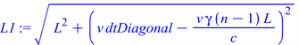
The diagonal distance L₁ can be calculated by subtracting the horizontal distance travelled by the gas molecules during the time that the light is absorbed by them.

$c_n=\frac{c}{n}$

$\text{Fraction Of Time Light Is Held By Molecules}=\frac{n-1}{n}$

$\begin{array}{l}\text{Time Light Is Held By Molecules}\\ =\gamma \cdot \text{Fraction Of Time Light Is Held By Molecules}\cdot \frac{L}{c_n}\end{array}$

$t_0=\frac{L}{c_n}$

$L_1=\sqrt{L^2+{\left(v\cdot d{t}_{\text{Diagonal}}-v\cdot \text{Time Light Is Held By Molecules}\right)}^2}$

$d{t}_{\text{Diagonal}}=t_0+\left(\frac{L_1-L}{c}\right)$

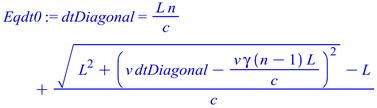
t₀ is the time it takes light to cross the distance (through the air) in the interferometer arm when it is at rest.

c_n is the reduced speed of light due to the higher refractive index of the air (c/n)

L₁ is the actual distance (through the Aether) that the light travels as it goes from one end of the (perpendicular) interferometer arm to the other (when the interferometer is moving from the right to the left through the Aether).

dt_Diagonal is the time it takes the light to travel the distance L₁ meters plus the time that the light is held by the molecules. It is the time it takes light to travel a distance of L meters through air (t₀, which includes the time that the light is held by the air molecules) plus the time taken for the extra vacuum (Aether) due to the interferometer’s motion through the Aether’s frame (as light propagates at c relative to the Aether’s frame).

Time Light Is Held By Molecules is the period of time that the light is absorbed (and carried by) the optical medium molecules. During this time, it is not propagating through space at c.

If this timing equation for the perpendicular interferometer arm is then used in conjunction with the equation for the perpendicular arm (shown earlier) to model the experimental conditions of the Michelson-Morley and Miller (Mt Wilson) experiments, then we see that the predicted fringe shifts of the light in these interferometers are almost exactly the same as what was actually measured and recorded. See the Appendix of this paper for the mathematical model for these experiments and for a vacuum-mode setup using these same equations, which should (and does) yield a fringe shift expectation of zero.

4. Conclusions

In the quest to detect light speed anisotropy using interferometers it has been shown that a vacuum-mode interferometer is incapable of revealing if there is a light speed anisotropy in the reference frame of the interferometer. This is due to a cancelling of the timing differences caused by two different effects that occur simultaneously when the interferometer’s reference frame is in motion through space (the Aether field). These two effects are: 1) The changed optical path length; 2) The contracted length of the interferometer in the direction of motion.

However, despite this, when an optical medium (such as a gas) is introduced into the optical path in the interferometer, the calculations of the light path timing are altered such that they do not quite have the same values in the parallel and perpendicular interferometer arm directions. This makes detecting the light speed anisotropy that exists in the moving interferometer’s reference frame possible, although the timing difference is quite small. The resulting calculations, when applied to the experimental conditions used in the historical Michelson-Morley and Miller Mt Wilson experiments, reveal a predicted interference fringe shift in the interferometers that matches the actual, recorded experimental observations from these two experiments remarkably well.

So, despite the original conclusion that there is no Aether, drawn from these much-smaller-than-expected experimental results, this modelling reveals that the observed fringe shifts are exactly as would be expected from a light speed anisotropy in the interferometer’s reference frame caused by the existence of a preferred Aether reference frame. These modelled predictions are also in accord with the accurate Doppler shift anomalies of spacecraft Earth fly-bys measured by NASA [10] and interpreted as a light speed anisotropy in the Earth’s reference frame by Cahill [6]. He performed a detailed analysis of the various spacecraft Doppler anomalies and calculated a best-fit Aether wind speed for the Earth’s reference frame of ~486 km/s.

Appendix

The following pages show the mathematical model and resulting fringe shift prediction graphs (using the above gas-mode interferometer calculations) for the Michelson-Morley (FigureA1) and Miller (FigureA2) experiments, followed by the vacuum-mode case (FigureA3) where the refractive index is exactly 1. Each has a graph depicting the expected fringe shift at different Aether wind speeds (in 100’s of km/s). A Blue point is marked showing where the 486 km/s point is on the graph. This is the point representing the NASA Doppler shift measurements as interpreted by Cahill [6] as an Aether wind speed of ~486 km/s.

Appendix A. The Michelson-Morley Experiment Modelled

Figure A1. This graph shows the expected fringe shift in the interferometer on the Y-axis for a speed through the Aether (space) field of the magnitude shown on the X-axis (in km/sec) for the experimental setup used in the Michelson-Morley experiment of 1887.

Appendix B. The Miller Mt Wilson Experiment Modelled

Figure A2. This graph shows the expected fringe shift in the interferometer on the Y-axis for a speed through the Aether (space) field of the magnitude shown on the X-axis (in km/sec) for the experimental setup used in the Miller Mt Wilson experiment in 1933.

Appendix C. The Vacuum-Mode Interferometer Experiment

Figure A3. This graph shows the expected fringe shift in the interferometer on the Y-axis for a speed through the Aether (space) field of the magnitude shown on the X-axis (in km/sec) for a vacuum mode interferometer. Note that there is no fringe shift expected for a vacuum mode interferometer. Note: Due to calculation inaccuracy the calculated fringe shift is not exactly zero here, but the calculated number gets smaller according to the number of digits of precision used. Here I have used 200 digits and the calculated fringe shift is in the order of 10E−193. If the number of digits of precision is increased, this calculated fringe shift asymptotes to zero as expected.

Conflicts of Interest

The author declares no conflicts of interest regarding the publication of this paper.

References

[1]	Michelson, A. and Morley, E. (1887) On the Relative Motion of the Earth and the Luminiferous Ether. American Journal of Science, 34, 333-345. https://doi.org/10.2475/ajs.s3-34.203.333
[2]	Miller, D. (1933) The Ether-Drift Experiment and the Determination of the Absolute Motion of the Earth. Reviews of Modern Physics, 5, 203-242. https://doi.org/10.1103/RevModPhys.5.203
[3]	Miller, D.C. (1925) Ether-Drift Experiments at Mount Wilson. Nature, 116, 49-50. https://www.nature.com/articles/116049a0#citeas https://doi.org/10.1038/116049a0
[4]	Traill, D.A. (2012) A Classical Reconstruction of Relativity. https://www.researchgate.net/publication/343975995_A_Classical_Reconstruction_of_Relativity
[5]	Traill, D. (2021) Fresnel Dragging Explained by a Classical Model of Light Transmission in Optical Media. Journal of Applied Mathematics and Physics, 9, 1883-1889. https://doi.org/10.4236/jamp.2021.98121
[6]	Cahill R.T. (2009) Combining NASA/JPL One-Way Optical-Fiber Light-Speed Data with Spacecraft Earth-Flyby Doppler-Shift Data to Characterise 3-Space Flow. Progress in Physics, 4, 50-64. https://www.researchgate.net/publication/26842358_Combining_NASAJPL_One-Way_Optical-Fiber_Light-Speed_Data_with_Spacecraft_Earth-Flyby_Doppler-Shift_Data_to_Characterise_3-Space_Flow
[7]	Traill, D.A. (2021) Light Speed Anisotropy Experiment Using Coaxial Cables with Different Refractive Indices. https://www.researchgate.net/publication/354945033_Light_Speed_Anisotropy_experiment_using_Coaxial_cables_with_different_refractive_indices
[8]	Wikipedia (n.d.) Michelson-Morley Experiment. https://en.wikipedia.org/wiki/Michelson%E2%80%93Morley_experiment#cite_note-mill-58
[9]	Traill, D.A. (2021) The Parallel Interferometer Arm Light Timing Measurement. https://www.researchgate.net/publication/356161207_The_Parallel_interferometer_arm_light_timing_measurement
[10]	Anderson, J.D., Campbell, J.K., Ekelund, J.E., Ellis, J. and Jordan, J.F. (2008) Anomalous Orbital-Energy Changes Observed during Spacecraft Flybys of Earth. Physical Review Letters, 100, Article ID: 091102. https://journals.aps.org/prl/abstract/10.1103/PhysRevLett.100.091102 https://doi.org/10.1103/PhysRevLett.100.091102