Two Theorems of Multiple G-Itô Integral under G-Lévy Process

Hong Zheng, Yifei Xin

University of Shanghai for Science and Technology, Shanghai, China.

DOI: 10.4236/jamp.2022.102019                

Abstract

In this paper, according to G-Brownian motion and other related concepts and properties, we define multiple Itô integrals driven by G-Brownian motion and G-Lévy process. By using the G-Itô formula and the properties of G-expectation, two main theorems about Itô integral are obtained and proved. These two theorems provide powerful help for the subsequent research on jump process.

Keywords

G-Brownian Motion, G-Lévy Process, G-Itô Formula

1. Introduction

In recent years, nonlinear expectation theory has been applied more and more widely in the financial field. It can not only solve many uncertain problems in the financial field, but also has almost all the properties of classical mathematical expectation except linearity. In 2006, Peng [1] proposed the concepts of G-normal distribution G-expectation and G-Brownian motion, and established a complete theoretical framework. In 2008, Peng [2] proved the central limit theorem and the law of large numbers under sublinear expectations. Moreover, Peng [3] studied the existence and uniqueness of solutions of stochastic differential equations driven by G-Brownian motion under Lipschitz condition. In 2009, Peng and Hu [4] [5] studied more general nonlinear independent stationary incremental processes, especially nonlinear Lévy processes involving jump processes, and obtained the Representation theorem of G-expectation by Kolmogorov method under nonlinear expectations. In 2010, Peng [6] proposed the nonlinear expectation of backward stochastic differential equations and other applications. In 2013, Ren [7] proved the representation theorem for G-Lévy processes. Subsequently, Lin [8] introduces the stochastic integral of the increment process in the nonlinear expectation frame, and obtains the well-fitting theory of the solution of the reflection stochastic differential equation driven by G-Brown motion. In 2014, Geng et al. [9] developed G-SDE’s orbital analysis theory through rough-Path theory. Based on the development of nonlinear stochastic differential equation theory, Gao and Jiang [10] studied the large deviation problem of G-stochastic differential equation, and Gao and Xu [11] gave the concept of relative entropy in the framework of c expectation, thus establishing the principle of large deviation of empirical measures of independent random variables in the framework of sublinear expectation. Liu [12] studied some properties of multiple G-Itô integrals in G-expectation space. More information about G-expectations can be found in the literature [13] .

In this paper, we first give some related concepts and lemmas, including G-Brownian motion and G-Lévy process, G-Itô formula and product formula, and then use the above concepts and lemmas to get the definition of multiple G-Itô integrals, and give the proof process and examples.

The remainder of this paper is organized as follows: In Section 2, we first give the definition and properties of nonlinear space, and then introduce some concepts and theorems related to G-Brownian motion. In Section 3, we define several Itô integrals driven by multidimensional G-Brownian motion and G-Lévy process, and give relevant proofs. Finally, some important formulas for calculating G-Itô multiple integrals are given.

2. Preliminaries and Notation

In this section, we will give concepts related to the G-Lévy process. More relevant theories can be found in references [1] [2] [3] . Let $\Omega$ be a given set, and a vector lattice $\mathcal{H}$ on $\Omega$ is a linear space consisting of real-valued functions defined on $\Omega$ , and the following conditions are satisfied: 1) The constant c of each real-valued function is in $\mathcal{H}$ ; 2) if $X(\cdot )\in \mathcal{H}$ , also to have $\left|X(\cdot )\right|\in \mathcal{H}$ . The function in $\mathcal{H}$ is called the random variable, and the binary $\left(\Omega \mathrm{,}\mathcal{H}\right)$ is called the random variable space. A nonlinear expectation $\mathbb{E}$ is a function defined on the space H of random variables that satisfies the following four properties $\mathbb{E}\mathrm{<mo>\; :\; </mo>}\mathcal{H}\mapsto ℝ$ : 1) Monotonicity; 2) Preserving of constants; 3) Sub-additivity; 4) Positive homogeneity. The term triple $\left(\Omega \mathrm{,}\mathcal{H}\mathrm{,}\mathbb{E}\right)$ a nonlinear expectation space.

G-Brownian Motion and G-Lévy Process

Definition 1. [1] (G-Brownian motion) If for every $n\in \mathbb{N}$ and $0\le t_1,\cdots ,t_n<\infty$ , the following properties are satisfied:

1) $W_0\left(\omega \right)=0$ ;

2) The increment of $\left(W_t\right)$ is smooth and independent.

We call the random process $W_t\left(\omega \right)\left(t\ge 0\right)$ defined in a sublinear expectation $\left(\Omega \mathrm{,}\mathcal{H}\mathrm{,}\mathbb{E}\right)$ space for the Brown motion of $\mathbb{E}$ .

Definition 2. [14] (G-Lévy process) Let ${\left(X_t\right)}_{t\ge 0}$ be the d dimensional càdlàg process on a sublinear expectation space $\left(\Omega \mathrm{,}\mathcal{H}\mathrm{,}\mathbb{E}\right)$ . If $X_t$ satisfies the following properties, then $X_t$ is said to be G-Lévy process.

1) $X_0=0$ ;

2) Independent increments: for each $t,s\ge 0$ the increment $X_{t+s}-X_t$ is independent;

3) Stationary increments: the distribution of the increments $X_{t+s}-X_t$ is stable and does not depend on t;

4) for each $t\ge 0$ , $X_t=X_t^c+X_t^d$ ;

5) Two processes $X^c$ and $X^d$ satisfy the following conditions ${\lim }_{t\downarrow 0}\mathbb{E}\left[{\left|X_t^c\right|}^3\right]t^{-1}=0$ ; $\mathbb{E}\left[\left|X_t^d\right|\right]<Ct$ for all $t\ge 0$ .

Definition 3. [15] [16] (Poisson process) Let $\mathcal{V}:=\{v\in \mathcal{M}\left({ℝ}_0^d\right):\exists \left(p,q\right)\in {ℝ}^d\times {ℝ}^{d\times d}$ such that $\left(v\mathrm{,}p\mathrm{,}q\right)\in \mathcal{U}\}$ , Suppose there is a measure $\mu \in \mathcal{M}\left({ℝ}^d\right)$ such that ${\displaystyle {\int }_{{ℝ}_0^d}}\left|z\right|\mu \left(\text{d}z\right)<\infty$ and $\mu \left(\left\{0\right\}\right)=0$ . If $\lambda :={\sup }_{v\in \mathcal{V}}v\left({ℝ}_0^d\right)<\infty$ , let’s say G-Lévy process X is a finite activity G-Lévy process X. When $d=1$ , the Lebesgue measure on the interval $\left[\mathrm{0,}\lambda \right]$ is $\mu$ and $g_v:=F_v^{-1}$ , Where $F_v^{-1}$ is the inverse of $F_v$ . When $d>1$ , consider the Knothe-Rosenblatt rearrangement to transport measure $\mu$ and measure v, More details in reference. Consider $\left(\Omega \mathrm{,}\mathcal{H}\mathrm{,}\mathbb{E}\right)$ be a probability space, it has a Brownian motion W and a Lévy process, which is independent of W. We define $N_t={\displaystyle {\int }_{{ℝ}_0^d}}xN\left(t\mathrm{,}\text{d}x\right)$ in the finite activity case $\lambda ={\sup }_{v\in \mathcal{V}}v\left({ℝ}_0^d\right)<\infty$ define the Poisson process M with intensity $\lambda$ by putting $M_t=N\left(t,{ℝ}_0^d\right)$ .

Definition 4. [3] We first consider the quadratic variation process of one-dimensional G-Brownian motion ${\left(W_t\right)}_{t\ge 0}$ with $W_1\doteq N\left(\left\{0\right\}\times \left[{\underset{\_}{\sigma }}^2,{\bar{\sigma }}^2\right]\right)$ . Let ${\pi }_t^N,N=1,2,\cdots$ be a sequence of partitions of $\left[\mathrm{0,}t\right]$ . We consider

$W_t^2={\displaystyle \underset{j=0}{\overset{N-1}{\sum }}}\left(W_{t_{j+1}^N}^2-W_{t_j^N}^2\right)={\displaystyle \underset{j=0}{\overset{N-1}{\sum }}}2W_{t_j^N}\left(W_{t_{j+1}^N}-W_{t_j^N}\right)+{\displaystyle \underset{j=0}{\overset{N-1}{\sum }}}{\left(W_{t_{j+1}^N}-W_{t_j^N}\right)}^2.$

As $\mu \left({\pi }_t^N\right)\to 0$ , the first term of the right side converges to $2{\displaystyle {\int }_0^t}{W}_s\text{d}{W}_s$ in $L_G^2\left(\Omega \right)$ . The second term must be convergent. We denote its limit by ${\langle W\rangle }_t$ , i.e.,

${\langle W\rangle }_t:=\underset{\mu \left({\pi }_t^N\right)\to 0}{lim}{\displaystyle \underset{j=0}{\overset{N-1}{\sum }}}{\left(W_{t_{j+1}^N}-W_{t_j^N}\right)}^2=W_t^2-2{\displaystyle {\int }_0^t}{W}_s\text{d}{W}_s.$

By the above construction, ${\left({\langle W\rangle }_t\right)}_{t\ge 0}$ is an increasing process with ${\langle W\rangle }_0=0$ . We call it the quadratic variation process of the G-Brownian motion.

Next, we will give two important lemmas under G-Lévy process.

Lemma 1. [1] (G-Itô formula) We denote $W_t$ be a m-dimensional G-Brownina motion. Let $g\in C^2\left({ℝ}^d\right)$ be bounded with bounded derivatives and $\frac{{\partial }^{2}g}{\partial x^i\partial x^j}$ are uniformly Lipschitz. Let $s\in \left[\mathrm{0,}T\right]$ be fixed and let $X_t^i$ be the i-th component of $X_t={\left(X_t^1\mathrm{,}\cdots \mathrm{,}{X}_t^d\right)}^{\text{T}}$ satisfying

$X_t^i=X_0^i+{\displaystyle {\int }_0^t}{a}_s^i\text{d}s+{\displaystyle \underset{j=1}{\overset{m}{\sum }}}{\displaystyle {\int }_0^t}{\eta }_s^{i,j}\text{d}{\langle W\rangle }_s^j+{\displaystyle \underset{j=1}{\overset{m}{\sum }}}{\displaystyle {\int }_0^t}{\sigma }_s^{i,j}\text{d}{W}_s^j+{\displaystyle {\int }_0^t}{\displaystyle {\int }_{\mathcal{E}}}c\left(e,s\right)N\left(\text{d}e,\text{d}s\right),$

where $a^i$ be the i-th of $a={\left(a^1\mathrm{,}\cdots \mathrm{,}{a}^d\right)}^{\text{T}}$ , ${\eta }^{i\mathrm{,}j}$ and ${\sigma }^{i\mathrm{,}j}$ is the lines i-th and j-th of $\eta ={\left({\eta }^{i\mathrm{,}j}\right)}_{d\times m}$ and $\sigma ={\left({\sigma }^{i\mathrm{,}j}\right)}_{d\times m}$ . Let $W_t=\left(W_t^1\mathrm{,}\cdots \mathrm{,}{W}_t^m\right)$ is m-dimensional G-Brownian and $N_t$ G-Lévy process, we have

$\begin{array}{l}g\left(X_t\right)-g\left(X_0\right)\\ ={\displaystyle \underset{i=1}{\overset{d}{\sum }}}\left[{\displaystyle {\int }_0^t}\frac{\partial g}{\partial x^i}\left(X_s\right)a_s^i\text{d}s+{\displaystyle \underset{j=1}{\overset{m}{\sum }}}{\displaystyle {\int }_0^t}\frac{\partial g}{\partial x^i}\left(X_s\right){\sigma }_s^{i,j}\text{d}{W}_s^j\right]\\ +{\displaystyle {\int }_0^t}\left[{\displaystyle \underset{i=1}{\overset{d}{\sum }}}{\displaystyle \underset{j=1}{\overset{m}{\sum }}}\frac{\partial g}{\partial x^i}\left(X_s\right){\eta }_s^{i,j}+\frac{1}{2}{\displaystyle \underset{i,l=1}{\overset{d}{\sum }}}{\displaystyle \underset{j=1}{\overset{m}{\sum }}}\frac{{\partial }^{2}g}{\partial x^i\partial x^j}\left(X_s\right){\sigma }_s^{i,j}{\sigma }_s^{l,j}\right]\text{d}{\langle W\rangle }_s^j\\ +{\displaystyle {\int }_0^t}{\displaystyle {\int }_{\mathcal{E}}}\left[g\left(X_{s-}+c\left(e\mathrm{,}s\right)\right)-g\left(X_{s-}\right)\right]N\left(\text{d}e\mathrm{,}\text{d}s\right).\end{array}$

Lemma 2. (Product rule) [1] For the m-dimensional G-Brownian and one-dimensional G-Lévy jump process, according to G-Itô formula, we have the following result as follows:

$\begin{array}{l}\text{d}{W}_t^i\text{d}{W}_t^j=0,i\ne j;\text{d}{W}_t^i\text{d}{W}_t^i=\text{d}{\langle W\rangle }_t^i;\text{d}t\text{d}{N}_t=0;\\ \text{d}{N}_t\text{d}{W}_t^i=0;\text{d}{N}_t\text{d}{N}_t=\lambda \left(\text{d}e\right)\text{d}t+{\left(\lambda \left(\text{d}e\right)\right)}^2\text{d}t.\end{array}$

where $1\le i\mathrm{,}j\le m$ , $i\ne j$ .

3. Main Results

In this section, we will introduce two theorems of the multi-dimensional G-Itô integral under G-Lévy process. We firstly give the definition of multiple G-Itô integral $I_{\alpha }{\left[f(\cdot )\right]}_{t_n\mathrm{,}{t}_{n+1}}$ . Then we will introduce two theorems.

We shall call a row vector $\alpha =\left(j_1\mathrm{,}{j}_2\mathrm{,}\cdots \mathrm{,}{j}_l\right)$ , where $j_i\in \left\{-\mathrm{1,}\cdots \mathrm{,2}m\right\}$ , $i\in \left\{\mathrm{1,2,}\cdots \mathrm{,}l\right\}$ and $l=1,2,3,\cdots$ . We define a multi-index of length $l:=l\left(\alpha \right)\in \left\{1,2,\cdots \right\}$ . Moreover, $\alpha -$ and $-\alpha$ denote the multi-index that deletes the first and last component of $\alpha$ . Next, we denote the set of all multi-indices by $\mathcal{M}$

$\mathcal{M}=\left\{\left(j_1,j_2,\cdots ,j_l\right):j_i\in \left\{-1,\cdots ,2m\right\},l\in \left\{1,2,3,\cdots \right\}\right\}\cup \left\{v\right\},$

where v is the multi-index of length zero.

Definition 5. For $0\le t_n\le s\le t_{n+1}\le T$ and $\alpha \in \mathcal{M}$ , we introduce the definition of multiple G-Itô integral $I_{\alpha }{\left[f(\cdot )\right]}_{t_n\mathrm{,}{t}_{n+1}}$ as follows:

$I_{\alpha }{\left[f(\cdot )\right]}_{t_n,t_{n+1}}=\{\begin{array}{ll}f\left(s\right),\hfill & \text{if}l=0\hfill \\ {\displaystyle {\int }_{t_n}^{t_{n+1}}}{I}_{\alpha -}{\left[f(\cdot )\right]}_{t_n,s_l}\text{d}{G}_{s_l}^{j_l},\hfill & \text{if}l\ge 1\text{and}-1\le j_l\le 2m,\hfill \end{array}$

where $G_t^0=t$ , $G_t^i=W_t^i$ is G-Brownian motion for $1\le i\le m$ , $G_t^j={\langle W\rangle }_t^{j-m}$ for $m+1\le j\le 2m$ , $G_t^{-1}={\tilde{N}}_t$ is a compensated G-Lévy jump process.

By using the Definition 5, we have the following result as follows:

$\begin{array}{l}{I}_{\left(2,0\right)}{\left[f(\cdot )\right]}_{t_n,t_{n+1}}={\displaystyle {\int }_{t_n}^{t_{n+1}}}{\displaystyle {\int }_{t_n}^{s_2}}f\left(s_1\right)\text{d}{W}_{s_1}^2\text{d}{s}_2,\\ I_{\left(0,m+1\right)}{\left[f(\cdot )\right]}_{t_n,t_{n+1}}={\displaystyle {\int }_{t_n}^{t_{n+1}}}{\displaystyle {\int }_{t_n}^{s_2}}f\left(s_1\right)\text{d}{s}_1\text{d}{\langle W\rangle }_{s_2}^1,\end{array}$

$\begin{array}{l}{I}_{\left(2,-1\right)}{\left[f(\cdot )\right]}_{t_n,t_{n+1}}={\displaystyle {\int }_{t_n}^{t_{n+1}}}{\displaystyle {\int }_{t_n}^{s_2}}f\left(s_1\right)\text{d}{W}_{s_1}^2\text{d}{\tilde{N}}_{s_2},\\ I_{\left(0,-1\right)}{\left[f(\cdot )\right]}_{t_n,t_{n+1}}={\displaystyle {\int }_{t_n}^{t_{n+1}}}{\displaystyle {\int }_{t_n}^{s_2}}f\left(s_1\right)\text{d}{s}_1\text{d}{\tilde{N}}_{s_2}.\end{array}$

For the simple of theorem proving, we define some notation such as $I_{\alpha ,s}=I_{\alpha }{\left[1\right]}_{0,s}$ and $W_s^0=s$ for $\alpha \in \mathcal{M}\mathrm{,}s\ge 0$ . Next, we will introduce two theories under G-Lévy process.

Theorem 1. For multi-index ${\alpha }^n=\left(j_1,j_2,\cdots ,j_n\right),-1\le j_i\le 2m$ ( $j_i\in \mathbb{Z}$ ), and $j_1\mathrm{,}{j}_2\mathrm{,}\cdots \mathrm{,}{j}_n$ are not equal with each other. The set $C\left({\alpha }^n\right)$ be the all of the n level arrangement of ${\alpha }^n$ , define

$C\left({\alpha }^n\right)=\left\{\left(a_1,a_2,\cdots ,a_n\right)|a_i\in \left\{j_1,j_2,\cdots ,j_n\right\},i=1,\cdots ,n,2\le n\le m\right\},$

such that

$H_{C\left({\alpha }^n\right)}={\displaystyle \underset{\alpha \in C\left({\alpha }^n\right)}{\sum }}{I}_{\alpha ,t}={\displaystyle \underset{i=1}{\overset{n}{\prod }}}{G}_t^{j_i}.$

Proof. For $n=2$ , we have $I_{\left(i,j\right),t}+I_{\left(j,i\right),t}={\displaystyle {\int }_0^t}{\displaystyle {\int }_0^s}\text{d}{G}_r^i\text{d}{G}_s^j+{\displaystyle {\int }_0^t}{\displaystyle {\int }_0^s}\text{d}{G}_r^j\text{d}{G}_s^i=G_t^i{G}_t^j$ ;

For $n=k$ we have $H_{C\left({\alpha }^k\right)}={\displaystyle \underset{\alpha \in C\left({\alpha }^k\right)}{\sum }}{I}_{\alpha ,t}={\displaystyle {\prod }_{i=1}^k}{G}_t^{j_i}$ . We need to prove that

$H_{C\left({\alpha }^{k+1}\right)}={\displaystyle \underset{\alpha \in C\left({\alpha }^{k+1}\right)}{\sum }}{I}_{\alpha ,t}={\displaystyle \underset{i=1}{\overset{k+1}{\prod }}}{G}_t^{j_i}.$

Actually, we only need to prove that

${\displaystyle \underset{l=1}{\overset{k+1}{\sum }}}{\displaystyle {\int }_0^t}{H}_{C\left({\alpha }^{k+1}-\left(j_l\right)\right),t}\text{d}{G}_t^{j_l}={\displaystyle \underset{l=1}{\overset{k+1}{\sum }}}{\displaystyle {\int }_0^t}{\displaystyle \underset{i=1,i\ne l}{\overset{k}{\prod }}}{G}_t^{j_i}\text{d}{G}_t^{j_l}={\displaystyle \underset{i=1}{\overset{k+1}{\prod }}}{G}_t^{j_i}.$ (1)

where $\alpha =\left(j_1\mathrm{,}{j}_2\mathrm{,}\cdots \mathrm{,}{j}_k\mathrm{,}j\right)$ and ${\alpha }^{k+1}-\left(j_l\right)$ for the k-index obtained by deleting the last component $j_l$ of ${\alpha }^{k+1}$ . In fact, applying G-Itô formula and independence of Brown motion, one has

$\text{d}{\displaystyle \underset{i=1}{\overset{k+1}{\prod }}}{G}_t^{j_i}={\displaystyle \underset{l=1}{\overset{k+1}{\sum }}}{\displaystyle \underset{i=1,i\ne l}{\overset{k}{\prod }}}{G}_t^{j_i}\text{d}{G}_t^{j_l}.$ (2)

Taking integral on Equation (2) and combined with Equation (1), the proof is completed. This theorem greatly simplifies the calculation process and provides some convenience for the subsequent related research.

Example. For $i\mathrm{,}j\mathrm{,}k\in \left\{\mathrm{1,2,3,}\cdots \mathrm{,}m\right\}$ , and $i\mathrm{,}j\mathrm{,}k$ are different from each other. Using G-Itô formula and the above theorem 1, we can get

$\begin{array}{l}{I}_{\left(i,j,k\right),t}+I_{\left(j,i,k\right),t}+I_{\left(k,i,j\right),t}+I_{\left(i,k,j\right),t}+I_{\left(k,j,i\right),t}+I_{\left(j,k,i\right),t}\\ ={\displaystyle {\int }_0^t}{G}_z^i{G}_z^j\text{d}{G}_z^k+{\displaystyle {\int }_0^t}{G}_z^k{G}_z^i\text{d}{G}_z^j+{\displaystyle {\int }_0^t}{G}_z^k{G}_z^j\text{d}{G}_z^i\\ =G_t^i{G}_t^j{G}_t^k.\end{array}$

There is a recursive relationship for multiple G-Itô integrals, which we shall now derive.

Theorem 2. Given on a sublinear expectation space $\left(\Omega \mathrm{,}\mathcal{H}\mathrm{,}\mathbb{E}\right)$ , $N_t={\displaystyle {\sum }_{s\in \left(0,t\right]}}\Delta N_s$ . We have

${\displaystyle {\int }_{\left(0,t\right]}}{\displaystyle {\int }_{\left(0,s_1\right)}}\cdots {\displaystyle {\int }_{\left(0,s_{n-1}\right)}}\text{d}{N}_{s_1}\cdots \text{d}{N}_{s_{n-1}}\text{d}{N}_{s_n}=\{\begin{array}{ll}\left(\begin{array}{c}{N}_t\\ n\end{array}\right)\hfill & \text{for}{N}_t\ge n\hfill \\ 0\hfill & \text{otherwise}\hfill \end{array}$

for $t\in \left[\mathrm{0,}T\right]$ , where

$\left(\begin{array}{c}i\\ n\end{array}\right)=\frac{i!}{n!\left(i-n\right)!}$

for $i\ge n$ .

Proof. We prove it by mathematical induction. For $n=1$ , we have ${\displaystyle {\int }_{\left(0,t\right]}}\text{d}{N}_s=N_t$ ;

For $n=2$ , according to G-Itô formula above, we can get ${\displaystyle {\int }_{\left(0,t\right]}}{\displaystyle {\int }_{\left(0,s_1\right)}}\text{d}{N}_{s_1}\text{d}{N}_{s_2}=\frac{1}{2!}{N}_t\left(N_t-1\right)$ ;

For $n=k$ , we have ${\displaystyle {\int }_{\left(0,t\right]}}{\displaystyle {\int }_{\left(0,s_1\right)}}\cdots {\displaystyle {\int }_{\left(0,s_{k-1}\right)}}\text{d}{N}_{s_1}\cdots \text{d}{N}_{s_{k-1}}\text{d}{N}_{s_k}=\left(\begin{array}{c}{N}_t\\ k\end{array}\right)$ , for $N_t\ge k$ . We need to prove that

$\begin{array}{l}{\displaystyle {\int }_{\left(0,t\right]}}{\displaystyle {\int }_{\left(0,s_1\right)}}\cdots {\displaystyle {\int }_{\left(0,s_k\right)}}\text{d}{N}_{s_1}\cdots \text{d}{N}_{s_k}\text{d}{N}_{s_{k+1}}\\ ={\displaystyle {\int }_{\left(0,t\right]}}\left(\begin{array}{c}{N}_{s_1}\\ k\end{array}\right)\text{d}{N}_{s_{k+1}}={\displaystyle {\int }_{\left(0,t\right]}}\left(\begin{array}{c}{N}_{s_1+1}\\ k+1\end{array}\right)-\left(\begin{array}{c}{N}_{s_1}\\ k+1\end{array}\right)\text{d}{N}_{s_{k+1}}=\left(\begin{array}{c}{N}_t\\ k+1\end{array}\right)\end{array}$

According to mathematical induction and G-Itô formula, the proof is completed.

The above theorems can help us to get the iterative formula of the jump process equation and provide beneficial help for the subsequent related research.

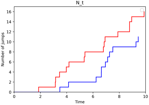
Numerical Simulation. The relevant numerical simulation is given below. In the G-expectation space, we consider the simulation of the G-Poisson process. It can be seen from the following figure that the G-Poisson process shows a phased rise, in which the red line segment is $\lambda =2t$ and the blue line segment is $\lambda =t$ .

Conflicts of Interest

The authors declare no conflicts of interest regarding the publication of this paper.

References

[1]	Peng, S. (2007) G-Expectation, G-Brownian Motion and Related Stochastic Calculus of Itô Type. In: Benth, F.E., Di Nunno, G., Lindstrøm, T., Øksendal, B. and Zhang, T., Eds., Stochastic Analysis and Applications, Springer, Berlin, Heidelberg, 541-567. https://doi.org/10.1007/978-3-540-70847-6_25
[2]	Peng, S. (2008) A New Central Limit Theorem under Sublinear Expectations.
[3]	Peng, S. (2010) Nonlinear Expectations and Stochastic Calculus under Uncertainty.
[4]	Hu, M. and Peng, S. (2009) G-Lévy Processes under Sublinear Expectations.
[5]	Hu, M. and Peng, S. (2009) On Representation Theorem of G-Expectations and Paths of G-Brownian Motion. Acta Mathematicae Applicatae Sinica, English Series, 25, 539-546. https://doi.org/10.1007/s10255-008-8831-1
[6]	Peng, S. (2010) Backward Stochastic Differential Equation, Nonlinear Expectation and Their Applications. Proceedings of the International Congress of Mathematicians 2010 (ICM 2010) (In 4 Volumes), Vol. I: Plenary Lectures and Ceremonies Vols. II–IV: Invited Lectures, 393-432.
[7]	Ren, L. (2013) On Representation Theorem of Sublinear Expectation Related to G-Lévyprocess and Paths of G-Lévy Process. Statistics & Probability Letters, 83, 1301-1310. https://doi.org/10.1016/j.spl.2013.01.031
[8]	Lin, Y. (2013) Stochastic Differential Equations Driven by G-Brownian Motion with Reflecting Boundary. Institute of Mathematical Statistics and Bernoulli Society, 18, 1-23. https://doi.org/10.1214/EJP.v18-2566
[9]	Geng, X., Qian, Z. and Yang, D. (2014) G-Brownian Motion as Rough Paths and Differential Equations Driven by G-Brownian Motion. In: Donati-Martin, C., Lejay, A. and Rouault, A., Eds., Séminaire de Probabilités XLVI, Springer, Cham, 125-193. https://doi.org/10.1007/978-3-319-11970-0_6
[10]	Gao, F. and Jiang, H. (2010) Large Deviations for Stochastic Differential Equations Driven by G-Brownian Motion. Stochastic Processes and Their Applications, 120, 2212-2240. https://doi.org/10.1016/j.spa.2010.06.007
[11]	Gao, F. and Xu, M. (2012) Relative Entropy and Large Deviations under Sublinear Expectation. Acta Mathematica Scientia, 32, 1826-1834. https://doi.org/10.1016/S0252-9602(12)60143-X
[12]	Liu, F. (2018) Some Important Properties of Multiple G-Itô Integral in the G-Expectation Space. Journal of Applied Mathematics and Physics, 6, 2219-2226. https://doi.org/10.4236/jamp.2018.611186
[13]	Peng, S. (2017) Theory, Method and Significance of Nonlinear Expectation. Scientia Sinica Mathematica, 47, 1223-1254. https://doi.org/10.1360/N012016-00209
[14]	Paczka, K. (2012) Itô Calculus and Jump Diffusions for G-Lévy Processes.
[15]	Wu, P. (2013) Multiple G-Itô Integral in G-Expectation Space. Frontiers of Mathematics in China, 8, 465-476. https://doi.org/10.1007/s11464-013-0288-8
[16]	Villani, C. (2009) Optimal Transport: Old and New. Springer, Berlin, Heidelberg. https://doi.org/10.1007/978-3-540-71050-9