Prediction of Protein Expression and Growth Rates by Supervised Machine Learning

Simiao Zhao

School of Informatics, University of Edinburgh, Edinburgh, United Kingdom.

DOI: 10.4236/ns.2021.138025                

Abstract

The DNA sequences of an organism play an important influence on its transcription and translation process, thus affecting its protein production and growth rate. Due to the com-plexity of DNA, it was extremely difficult to predict the macroscopic characteristics of or-ganisms. However, with the rapid development of machine learning in recent years, it be-comes possible to use powerful machine learning algorithms to process and analyze biolog-ical data. Based on the synthetic DNA sequences of a specific microbe, E. coli, I designed a process to predict its protein production and growth rate. By observing the properties of a data set constructed by previous work, I chose to use supervised learning regressors with encoded DNA sequences as input features to perform the predictions. After comparing different encoders and algorithms, I selected three encoders to encode the DNA sequences as inputs and trained seven different regressors to predict the outputs. The hy-per-parameters are optimized for three regressors which have the best potential prediction performance. Finally, I successfully predicted the protein production and growth rates, with the best R² score 0.55 and 0.77, respectively, by using encoders to catch the potential fea-tures from the DNA sequences.

Keywords

DNA Sequences, Protein Production, Growth Rate, Supervised Machine Learning

1. INTRODUCTION AND BACKGROUND LITERATURE

With the increasing applications of machine learning algorithms in biology, more and more recent researches of computational biology focused on analyzing DNA [1].

Deoxyribonucleic acid (DNA) is a biological macromolecule with a double helix structure (Figure 1). Its basic unit is deoxynucleotide. Each single nucleotide consists of three compounds, phosphoric acid, deoxyribose and nucleobase. The phosphoric acids and deoxyriboses are nearly the same for all nucleotides but the nucleobases are not. There are two types of nucleobase: purines and pyrimidines. Purines mainly include adenine (A) and guanine (G), and pyrimidines mainly include cytosine (C) and thymine

Figure 1. DNA structure [2].

(T). On the inner side of the double helix structure of the DNA molecule, the base pairs are formed by hydrogen bonds (A pairs with T, C pairs with G) so that the two long deoxynucleotide chains are firmly connected in parallel. Different kinds of nucleobase pairs promote the diversity of DNA molecules [3].

The function of DNA molecules is to store all the genetic information that determines the traits of a species. DNA controls the orderly transcription of genes in biological organisms, enables them to complete all the procedures of development, and ultimately determines the unique traits of organisms.

Organisms grow populations and synthesize proteins by translating the genetic information on messenger RNA (mRNA), and the mRNA is transcribed from DNA (Figure 2). Therefore, the growth rates and protein production of the organisms are greatly related to their DNA structures. If there is a method to predict the protein production and growth rates of a microorganism with its given DNA, it will greatly help researchers to understand or design DNA sequences [4].

Guillaume Cambray, Joao C Guimaraes and Adam Paul Arkin researched the influence of synthetic DNA sequences on the translation of a microbe, Escherichia coli in previous work [6]. A DNA sequence is a string of letters, which is used to represent the primary structure of a DNA molecule that carries genetic information. The primary structure of DNA refers to the linkage and arrangement sequence of the four deoxynucleotides. The only possible letters are A, C, G, and T, which represent the four nucleotides that make up DNA. Each nucleotide contains its corresponding base (adenine, cytosine, guanine, and thymine) (Figure 3). The line represents a sequence consists of different nucleotides. The promoter is a region of DNA where transcription of a gene is initiated, and the transcription stops at the transcription stop site.

In the previous research, researchers synthesized 244,000 different DNA sequences by varying the coding sequence part of the DNA sequence based on eight different features, which impacted on four important levels in transcription and translation process [6].

1) On nucleotide level, they considered the percentage of adenine-thymine bases in the synthetic DNA sequence.

2) On codons level, they considered the codon adaptation index (CAI). A codon is a sequence of three nucleotides which together form a unit of genetic code in a DNA molecule. CAI means how easy the codons can be translated to the basic unit of protein, amino acid. Bottleneck position and strength mean where and how strong the translation process gets stuck on a position of the sequence.

3) On the amino acids level, they considered the mean hydropathy index, which is how hydrophobic the amino acid is.

4) Finally, they considered the predicted minimum free energy (MFE) of the sequence string on the

Figure 2. DNA to protein process [5].

Figure 3. DNA sequence structure [7].

mRNA structures level. The free energy can be thought of as the energy released by folding a completely unfolded RNA molecule, and the minimum free energy structure of a sequence is the secondary structure which is created by nucleobases pairing and calculated to have the lowest value of free energy. The researchers considered the MFE of three parts of the sequence string. The first part of the string ranges from position [−30, 30] which is from the fixed thirtieth nucleotides before the start codon to the thirtieth designed nucleotides after the start codon. The second part of string ranges from [1, 60], which is from the first of the first designed nucleotides after the start codon to the sixtieth, and the third part of string ranges from [30, 90].

From the above considerations, they firstly generated 56 mother sequences which are different from each other as much as possible. For each of the mother sequence, they mutated until they obtained all combinations of the eight properties mentioned above. Then, they generated variants per sequence by introducing 1 - 4 nucleotides mutations to synthesize the 244,000 sequences and put each of them on a plasmid to transform the E. coli cells. The E. coli cells got different DNA sequences, and a population with the same DNA sequences is called a strain.

As the process in Figure 4 shows, the researchers leave these cells for a certain amount of time. In order to measure the protein production, they sorted the cells by fluorescence activating cell sorter (FACS), used polymerase Chain Reaction (PCR) to amplify the specific piece of DNA sequence, and finally deep-sequenced the DNA to obtain the green fluorescent protein (GFP) for each strain. Similarly, by measuring the difference between abundances before and after the time period with PCR and deep-sequencing techniques, they obtained the growth rate of each strain.

By measuring the green fluorescent protein and growth rates of all strains, they constructed a complete data set. They used the data set for analyzing how the translation efficiency is influenced by the transcript structures.

In my research, I applied the data set on predicting the protein production and growth rates from the synthetic DNA sequences. I selected 24,600 sequences as my research data set, which is a subset of the original data set. There are 24,600 rows, where each row is a sample, and 18 columns, where each column is a feature. My research only used 11 columns, other irrelevant columns, such as halflife, polysome value, and abundance value were discarded. The 11 columns contain the following information for each sample:

1) The 96 long synthetic DNA sequence

2) The protein production of the sample

3) The growth rate of the sample

4) The percentage of adenine-thymine bases

5) The bottleneck position

6) The bottleneck strength

7) The codon adaptation index

Figure 4. Process of GFP and growth rates measurement.

8) The mean hydropathy index

9) The predicted minimum free energy of first part of the string

10) The predicted minimum free energy of second part of the string

11) The predicted minimum free energy of third part of the string

Table 1 shows an example of above values in my data set, more details will be shown in data overview section in chapter three:

The metric I selected to evaluate my model performance is R-squared. R-squared (R²) is the measure of the extent that the variance of one variable explains the variance of the second variable. For example, if the R² of a model is 0.50, then approximately half of the observed variation can be explained by the model’s inputs. The formal definition will be given later in chapter two.

I implemented and compared the prediction performance of three different encoders, (one-hot encoder, k-mers overlapping encoder and k-mers non-overlapping Encoder), and seven different supervised machine learning algorithms. By using one-hot encoder to catch the potential features from the DNA sequences, I successfully predicted the protein production and growth rates of E. coli cells with best R-squared score 0.55 and 0.77, respectively, based on the synthetic DNA sequences.

2. DISCUSSION OF PROBLEMS AND SOLUTIONS

I encountered five problems during the experimental designing phase. They are:

1) Which features are selected as input features

2) If I choose to encode the DNA sequences into input features, which encoders are selected to encode the DNA sequences

3) Which algorithms are selected and how to build models

4) How much data is used for training and how much for validation and testing

5) Which metric is selected to judge my models

Most of the answers will be discussed in this chapter and some will be discussed in chapter three with experiment results for better illustration.

2.1. Feature Selection

There are two options for input features. One is to encode the DNA sequences in data set to obtain the input features, the other is to directly use the eight features mentioned in chapter one as input features.

Table 1. The examples of the values of columns.

In chapter three, I will discuss why the encoded DNA sequences are better input features for training models.

2.2. Encoder Selection

The sequences are strings constructed by four characters “A”, “T”, “C”, and “G”, these strings cannot be used directly for training models. An encoding method should be introduced to solve this problem. There are many genetic encoding methods can be chosen from.

1) Ordinal Encoder

This encoder assigns each nucleotide character with an ordinal number. It returns an array for an input of string. For example, string “ATGC” is encoded as [0, 1, 2, 3].

2) One-hot Encoder

This encoder is widely used in machine learning methods and is well suited to many machine learning algorithms. For example, the “ATGC” will become [[0, 0, 0, 1], [0, 0, 1, 0], [0, 1, 0, 0], [1, 0, 0, 0]]. The advantage of one-hot encoding is to ensure that machine learning models do not assume that higher numbers are more important. For example, a supervised learning model may regard G as a more important character than character T if the given string “ATGC” is encoded by ordinal encoder, but it will assume the two characters have the same importance if the string is encoded by one-hot encoder. This is because the model will assume 2 is heavier than 1, but assume [0, 0, 1, 0] and [0, 1, 0, 0] have the same weights. By using one-hot encoder, I could treat each nucleotide with the same importance. However, this method may ignore the potential relevance between each nucleotide, and it has higher time complexity for training models than ordinal encoder, since the dimensions of each nucleotide is four times more than dimensions of each nucleotide for ordinal encoder as shown in Table 2.

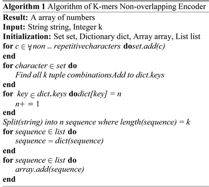
3) K-mers non-overlapping Encoder

The algorithm of k-mers non-overlapping Encoder is shown below.

Table 2. The results of encoding string “ATGC” by ordinal encoder and one-hot encoder.

Briefly, the encoder firstly learns all k-combinations of the given nucleotides in the string, and then assigns each of them with an ordinal number. Then it cuts a DNA sequence into N parts, with k nucleotides for each part. Finally, it assigns each part with the number that matches the combinations in the set.

This method significantly reduces the training time complexity, and retains the relevance of nucleotides in each sequence part. Also, when k = 1, it performs the same as ordinal encoding. However, there are several drawbacks. Firstly, the possible combinations increase exponentially with k. When k is large, it takes super long time to learn all the combinations as shown in Table 3. Secondly, it assumes different sequence parts have difference importance as mentioned previously for the ordinal encoder. Thirdly, it still ignores the relevance of each sequence parts. Finally, if k is not divisible by the original sequence length, then this k is not allowed and the k-mers non-overlapping encoder cannot be used [7].

4) K-mers Overlapping Encoder

The algorithm of k-mers overlapping encoder is shown below:

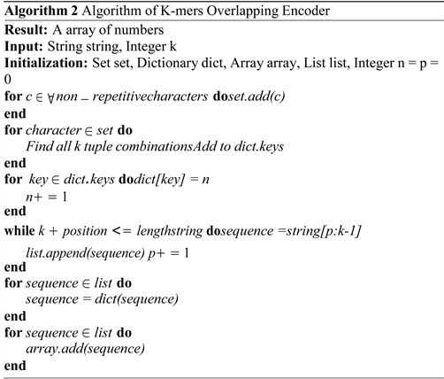
This method firstly learns all k combinations of the different nucleotides in the given DNA sequence and assigns each with an ordinal number to form a set. Then it breaks sequence into overlapping “words” of k-mers. For example, if I use 6-mers overlapping encoder on “ATGCATGCA”, it is broken into: “ATGCAT”, “TGCATG”, “GCATGC”, “CATGCA”. A sequence with length N to k-mers will have N-k+1 “words”. Finally, it assigns each part with the number that matchs the combinations in the set.

Table 3. Number of combinations when k increases.

It retains the correlation between every nucleotide as much as possible. However, it still suffers from learning high k combinations, and the importance assumption problem of ordinal encoder [8].

2.3. Algorithm Selection

1) Linear Regression (LR)

Linear regression is a statistical analysis method using regression analysis in mathematical statistics to determine the interdependent quantitative relationship between two or more variables, which is widely used. Its expression is:

$y=wx+b$

where b is the bias term, x is the input data, w is the weight, and y is the predicted output data [9].

2) Random Forest

Random forest is an ensemble learning method for classification, regression, and other tasks that operates by constructing multiple decision trees during training and out-putting classes as a pattern (classification) or average prediction (regression) of classes. Figure 5 shows the process of this algorithm.

The training data is splited into n bags, and each bag of data is used to train each decision trees. Finally, the regress or takes the mean of all trees and makes the prediction [11].

3) Multilayer Perceptrons (MLP)

Multilayer Perceptron (MLP) is a forward-structured artificial neural network that learns the function $f\left(x\right):R^I\to R^O$ , where I is the input feature dimensions and O is the output feature dimensions. Figure 6 shows a MLP with one hidden layer.

The input layer consists of neurons which are input features $\left[x_{\text{1}}\cdots x_n\right]$ . Each neuron in the hidden layer takes the values from the previous layer and transforms them with a weighted linear summation $w_{\text{1}}{x}_{\text{1}}+\cdots +w_m{x}_m$ , followed by a non-linear activation function $g\left(x\right):R\to R$ . In my research, I selected Relu as my activation function, which greatly accelerates the convergence of stochastic gradient descent compared with other activation function:

Figure 5. Random forest Regressor [10].

Figure 6. MLP with one hidden layer [12].

$f\left(x\right)=0$ if $x<0$

$f\left(x\right)=x$ if $x\ge 0$

MLP is capable to learn non-linear models, but it has a non-convex loss function where there exists more than one local minimum, and it takes longer time to be trained if the number of neurons and layers is large [13].

4) K Neighbors Regressor (KNN)

The principle of K Nearest Neighbor Regression is to find a predetermined number of points in the training sample that are closest to the new point and predict its value from these points. The number of these points is a defined constant. Distance can usually be measured in anyway. Standard euclidean distance is the most common choice [14]. The equation is shown below:

$d\left(p,q\right)=\sqrt{{\displaystyle \underset{i=1}{\overset{n}{\sum }}{q}_i-p_i^2}}$

where:

p, q = two points in Euclidean n-space

p_i, q_i = Euclidean vectors, starting from the origin of the space

n = n-space

5) Gradient Boosting Decision Tree Regressor (GBDT)

Gradient boosting decision tree regressor is an iterative decision tree algorithm [15]. GBDT algorithm can be regarded as an addition model composed of M trees, and its corresponding formula is as follows:

$F\left(x,w\right)={\displaystyle \underset{m=0}{\overset{M}{\sum }}{a}_m{h}_m\left(x,w_m\right)}={\displaystyle \underset{m=0}{\overset{M}{\sum }}{f}_m\left(x,w_m\right)}$

where:

x = the input samples

w = the model parameter

h = classified regression tree

a = the weight of each tree

F(x, w) = the prediction of regressor

1) Support Vector Regressor (SVR)

Support Vector Regression is an application of SVM (Support Vector Machine) to regression problem. SVR regression is to find a regression hyper-plane, so that all the data in a set have the closest distance to the plane.

The formula for SVR is:

$\begin{array}{l}\min \frac{1}{2}{\left|w\right|}^2+C{\displaystyle \underset{i=1}{\overset{n}{\sum }}\left|{\xi }_i\right|}\\ \text{Subjectto}\left|y_i-w_i{x}_i\right|\le \epsilon +\left|{\xi }_i\right|\end{array}$

where:

x = the input samples

w = the model parameter

y = the actual output value

ε = the distance from margin to hyperplane

C = the regularization parameter

ξ = the slack constant of margin tolerance

As shown in Figure 7, the traditional regression method considers the prediction correct when and only when the regression the output value f(x) is completely equal to y. However, for support vector regression, as long as f(x) and y are close, the prediction is regarded as a correct prediction. Specifically, the threshold value ε is defined, and only the loss of data points satisfy

$\left|f\left(x\right)-y\right|<\epsilon$ will be regarded as a correct prediction [17].

Different kernel functions can be applied on SVR to transform inputs into higher space so that it can fit non-linear distribution. However, I selected linear kernel because the models with linear assumption can be compared with other non-linear models for better illustration in chapter 3.

2) Voting Regressor (VR)

A voting regressor is an ensemble regressor that fits several basic regressors, each on the whole main data set. Then it averages the predictions of individual basic regressors to get a final prediction. I choose to set random forest and GBDT as the two basic regressors, since they have far better R² score than other algorithms in my experiments. The figures in chapter three will indicate that.

The algorithms above have different properties and performance on the data set. In chapter 3, I compared the performance of these algorithms and concluded random forest, GBDT and voting regressors are

Figure 7. SVR Hyper-plane [16].

the best and it is worth to search their hyper-parameters in a fine-grained grid.

2.4. Data Set Split

The proportions of training set, validation set and test set have huge impact on the training performance. If the training set is too small, the model will be trained with insufficient data, and may result in underfitting problem. However, since the size of whole data set is fixed, if the training set is too large, the size of validation set will be relative small to find the optimal hyper-parameters for the algorithms. Therefore, it is hard to decide the proper split sizes, where there is enough training data set and as much as possible validation data set. In chapter three, I compared the performance of various splits and got the best performance of model by splitting the data set into 80 percent training set and 20 percent validation and test set.

2.5. Metrics

There are three commonly used metrics to evaluate regression problems.

1) R-squared

R-squared (R²), for regression models, is a statistical measure of how much of variability in dependent variable can be explained by the model. In other words, R-squared is a statistical measure of how close the data are to the fitted regression line [18].

R-squared formula is:

$R^2=1-\frac{{\displaystyle {\sum }_{t=1}^n{\left(y_{true}-y_{pred}\right)}^2}}{{\displaystyle {\sum }_{t=1}^n{\left(y_{true}-y_{mean}\right)}^2}}$

where:

n = the number of data points

y_pred = the prediction value of model

y_true = the actual value

y_mean = the mean of actual value

The maximum of R² score is 1, and its value can be negative. The closer the predicted value of the model is to 1, the smaller the error of predicted value will be.

2) Mean Square Error (MSE)

MSE is widely used as metrics for regression problems in supervised machine learning. It is calculated by the sum of square of prediction error minus predicted output and then divided by the number of data points. It gives an absolute number on how much the predicted results deviate from the actual number [19].

Mean squared error formula is:

$\text{MSE}=\frac{1}{n}{\displaystyle \underset{t=1}{\overset{n}{\sum }}{\left(y_{true}-y_{pred}\right)}^2}$

n = number of data points

y_pred = the prediction value of model

y_true = the actual value

3) Mean Absolute Error (MAE)

MSE and MAE are similar. MAE is taking the mean of sum of absolute value of error, rather than the mean of sum of square error in MSE [20].

MAE formula is:

$\text{MAE}=\frac{1}{n}{\displaystyle \underset{t=1}{\overset{n}{\sum }}\left|y_{true}-y_{pred}\right|}$

n = number of data points

y_pred = the prediction value of model

y_true = the actual value

I selected R-squared as the evaluation metric of my models. This is because it takes the difference between the predicted value and the true value, as well as the variance among true values of the problem itself, into account. Also, it is convenient to use, since it is a built-in function in many python packages of supervised learning algorithms.

3. EXPERIMENTAL DESIGN AND IMPLEMENTATION

3.1. Data Overview

The huge amount of original 244,000 data set is too large for training a supervised machine learning model and may arouse high time complexity issue. Therefore, I used a subset of the original data set, which has 24,600 out of 244,000 sequences. The data set is combined with 6 seeds, each seed is originated from one of the 56 mother sequences described in chapter one. Each seed has the same combinations of sequence properties, but occupy a different place in the sequence space.

Each of the data sample contains the 96 long synthetic part of the DNA sequence, values of green fluorescent protein, values of relative growth rates, and values of eight properties, described in chapter one, for each of the E. coli cells. The ranges of these values are shown in Table 4.

Among the above values, values of protein production and growth rates are the actual output values for my research. Figure 8 and Figure 9 show the distribution of the measured values of protein production and growth rates of data.

The zig-zag distribution of protein values indicates that the values are irregularly distributed over the range. Moreover, the decrease of numbers when protein value is higher than 70 indicates that there are less E. coli cell samples which have high production of protein.

The growth rate distribution has a mountain shape, where it peaks at around 1.0. This means most of population of E. colis strains doubled after growing for a certain amount time mentioned in chapter one.

By plotting 2d histogram of protein production vs growth rate of the entire data set, the distribution and relationship between protein and growth rates of the E. coli cells can be obtained from Figure 10.

The growth rate firstly increases to a peak when the protein value is about 60 and then decreases when protein value increases continually. The convex curve may be because of the limited resources in

Table 4. The ranges of values of columns.

Figure 8. The distribution of protein values.

Figure 9. The distribution of growth rate values.

Figure 10. Protein values vs growth rates values.

microorganisms. Since ribosomes, minute particles that bind messenger RNA and transfer RNA to synthesize proteins, in organisms have limited amount, the excessive usage of ribosomes to produce protein may have adverse effects on their growth rate. This is mentioned in the previous research report of Guillaume Cambray, Joao C Guimaraes and Adam Paul Arkin [6].

3.2. Experiments

1) Feature Selection

In order to get more information about the relationship and characteristics of the eight features for designing the DNA sequences described in chapter one, I plotted the eight features against each other, it is shown in Figure 11.

Figure 11. Pairplot of eight properties.

As shown in the figure, most of the features are continuous, which means the possible values of these features can present at any point in the range. However, the bottleneck position has a polarization property. As shown in the figure, for bottleneck position vs itself, there are two data peaks existing on the two end of the possible range of values, which means, its values can appear in one of these two peaks only, and they are not possible to be any values between these two peaks. This feature may negatively impact on the prediction performance of protein production and growth rates. The reason is, since both the values of protein production and growth rate are continuous, for regression problem, it is hard for the model to find the inference between the continuous outcomes with the polarized features.

From Figure 12, the UMAP projection of the 8 features, which reduced the 8 dimensions of the 8 features to 2 dimensions, shows that the input data is divided into nearly two groups with the similar features. This is the demonstration of the influence of the polarized feature, bottleneck position. If the 8 features are directly used as input features, the predictions of protein and growth rates will tend to polarize, which will be different from the continuous distribution shown in Figure 8 and Figure 9.

For verification, I used the MLP and random forest algorithms to train models on the 8 features and the 4-mers non-overlapping encoded input features, respectively, with ten folds cross validations, for the same true values of protein. From Figure 13 and Figure 14, it can be seen that the R² score of the model using encoded synthetic DNA sequences as features is about 0.05 more than the model using the 8 features as input features. Therefore, I chose to use encoders to encode the DNA sequences into the input features rather than using the 8 features directly.

Figure 12. UMAP projection of eight properties.

Figure 13. The R² score with encoded DNA sequence input features by 4-mers non-overlapping encoder.

Figure 14. The R² score by using the eight properties as input features.

2) Encoders, Data split and Algorithm Selections

In order to find the best encoders, data split and algorithms described in chapter 2, I selected one seed, seed 37, from the six combined seeds, with 4191 data samples to perform experiments. By performing experiments on this smaller data set, I got the general trends and information about how the encoders, algorithms and data splits influence the performance of my models without fine-grained grid searching on a huge number of hyper-parameters or training the models for a long time. The distributions of the seed are shown in Figure 15 and Figure 16.

Figure 15. The distribution of protein values on selected seed.

Figure 16. The distribution of growth rate values on selected seed.

It is shown on the figures that the distributions of actual output values of the selected seed are similar to my whole data set. Therefore, it can be used as the experimental data set.

In my experiments, I firstly used different encoders to encode the DNA sequences in seed 37 into input features. Then, I trained different models with different data set splits by all the algorithms mentioned in chapter 2.

I grid searched the hyper-parameters coarsely for each algorithms so that the models can work well while do not cost long time for hyper-parameters searching. Table 5 shows the searched range and hyper-parameters with the best performance for models on different algorithms.

The meaning and function of each of the above hyper-parameters are explained below:

1) Max depth of random forest. Max depth represents the depth of each tree in the forest. The deeper the tree, the more splits it has and it captures more information about the data. However, if the tree is too deep, it may cause overfitting problem. This will be illustrated in chapter 4.

2) The hidden layers of MLP. Hidden layers are located between the input and output of MLP, perform nonlinear transformations of the inputs entered into the network as shown in Figure 6. Higher hidden layer number may improve the performance, but it also can cause overfitting problem.

3) The neurons of each hidden layer of MLP. The number of nodes in hidden layer is shown in 6.

4) The training epochs of MLP. The times of updating weights of MLP.

5) C of SVR. It is the regularization parameter. The strength of the regularization is inversely proportional to C.

6) Epsilon of SVR. The value of epsilon defines a margin of tolerance where no penalty is given to errors.

7) Max depth of GBDT. The maximum depth of regression estimators.

8) K in KNN regressor. It refers to the number of nearest neighbours to be included in the euclidean distance calculation mentioned in chapter 2.The hyper-parameters of linear regression algorithm and voting algorithm are not searched because their hyper-parameters will not influence the model performance in a significant scale.

For data splits experiments, I trained the models on training data splits from 10 percent to 90 percent, and used half of the rest data as validation set for hyper-parameters adjusting and half of it as test set for reporting the R² scores.

The protein production values in the data set are used as actual output values.

The best data split sizes, algorithms, encoders and hyper-parameters are the same as the models which use protein values as output values. However, generally, the performance of all models with all encoders is worse. This will be shown and explained in chapter 4.

a) One-hot Encoder with Different Splits of Data Size and Algorithms

Table 5. Hyper-parameters searching table.

As Figure 17 shows, when the size of test and validation split increases to more than 30 percent, the performance of all algorithms generally decrease. This is expected, because when the split size of training set decreases, the models are more tend to underfit.

Linear regression and SVR with linear kernel have the worst performance. Both of them take the same assumption that the DNA sequence and the protein production are linearly related. The result shows the assumption is wrong. The encoded DNA sequence attributes, because their high dimensionalities can cause many possible variations for the relationship between attributes and outputs, can easily break the assumption, which requires the output to linearly increase with each attribute. Non-linear regressor is required for the task.

KNN regressor and MLP perform not bad when enough training data is given. The best algorithms are random forest, GBDT, and voting with the random forest and GBDT basic regressors. Both random forest and GBDT are evolved version of decision tree regression algorithm, and decision tree regression is very suitable for this problem. The advantages of decision tree regression are:

a) It has faster training speed and prediction speed than other algorithms such as MLP.

b) It is good at acquiring nonlinear relation in data set.

c) It understands the characteristic interactions in data set.

d) It is good at dealing with outliers in data set.

e) It is good at finding the most important features in the data set.

f) It does not need feature scaling.

Overall, most regressors, with inputs encoded by one-hot encoder, perform well. The best R² score, 0.81, is achieved by random forest regressor with 90 percent training data split.

b) K-mers Non-overlapping Encoder with Different Splits of Data Size and Algorithms

In order to find the best k value for k-mers non-overlapping encoder, I performed experiments on values where k equals to 1, 2, 3, 4, 6, and 8. Since the sequence length is 96, the possible k values should be divisible by 96. Therefore, the values where k equals to 5, 7, and 9 cannot be experimented. As mentioned in encoder selection in chapter two, if k equals more than 9, the combinations to be learned by the encoder will be more than or equal to 2²⁰, which will cost long time to run and will not be a suitable encoder. The figures from 18 to 23 show the performance of different k-mers non-overlapping encoders.

Figure 18 shows that, for 1-mer non-overlapping encoder, the random forest, voting and GBDT are still the best algorithms for training models with R² score more than 0.7 when there are more than 70

Figure 17. Data split vs the R² score of seven models with one-hot encoder.

Figure 18. Data split vs the R² score of seven models with 1-mer non-overlapping encoder.

percent training data split. The best score, 0.78, is achieved by voting. The worst algorithms are still linear regression and SVR with linear kernel because of their linear assumptions. The overall scores of the best three algorithms are about 0.03 less than the scores of them for one-hot encoder. The general trend for data splits is nearly the same as the trend for one-hot encoder, where the performance decreases with the size of training set. The functions of 1-mer non-overlapping encoder and ordinal encoder are exactly the same according to the definition in encoder selection in chapter two, therefore, I did not experiment on ordinal encoder.

As Figure 19 shows, there are not much performance difference between 1-mer and 2-mers for non-overlapping encoders.

Except random forest, GBDT and voting algorithm, all algorithms have bad performance on 3-mers non-overlapping encoder. This problem may be caused by the algorithm of non-overlapping encoder mentioned in encoder selection of chapter two.

Since the string is cut into tuples with k characters, the relation between two different tuples cannot be retained. The bad performance in Figure 20 indicates that some potential relation between (3n)^th and (3n + 1)^th nucleotides, where n has range [1, 31], in the give DNA sequence is discarded by this encoder.

The performance of algorithms on 4-mers non-overlap encoder shown in Figure 21 is close to that on 1-mer, and 2-mers, and better than that on 3-mers. This indicates that the potential relation, which may be discarded in 3-mers non-overlapping encoder, is retained by 4-mers non-overlapping encoder.

As shown in Figure 22, The bad performance of both 3-mers and 6-mers non-overlapping encoders verified my assumption that there are some potential relation between (3n)^th and (3n + 1)^th nucleotides.

The performance of algorithms on 8-mers non-overlap encoder shown in Figure 23 is close to that on 1-mer, 2-mers, and 4-mers.

Generally, for k-mers non-overlapping encoders, where k = 1, 2, 4, and 8, the random forest, GBDT, and voting algorithms have the best R² scores which are more than 0.7. The advantages of decision tree based models are explained in last section. The best split size of test and validation set is about 30 percent. If it is more than 30 percent, the insufficient training set may lead to bad performance of models.

c) K-mers Overlapping Encoder with Different Splits of Data Size and Algorithms

In order to find the best k value for k-mers overlapping encoder, I performed experiments on values where k equals to 2, 3, 4, 6, and 8. The 1-mer overlapping encoder is exactly the same as 1-mer non-overlapping encoder according to the algorithms in encoder selection section of chapter 2. The

Figure 19. Data split vs the R² score of seven models with 2-mers non-overlapping encoder.

Figure 20. Data split vs the R² score of seven models with 3-mers non-overlapping encoder.

Figure 21. Data split vs the R² score of seven models with 4-mers non-overlapping encoder.

Figure 22. Data split vs the R² score of seven models with 6-mers non-overlapping encoder.

Figure 23. Data split vs the R² score of seven models with 8-mers non-overlapping encoder.

Figures 24-27 show the performance of different k-mers overlapping encoders.

The performance of models on 2-mers overlapping encoder shown in Figure 24 is close to that on one-hot encoder and better than that on non-overlapping encoders. This is because overlapping encoders retain the correlation between each nucleotide as much as possible. The best R² score, 0.81, is achieved by the model using voting algorithm.

Since overlapping encoders retain the correlation between each nucleotide as much as possible, 3-mers overlapping encoder performs much better than 3-mers non-overlapping encoder on all models. The best score is 0.79 of the model using voting algorithm, with 80 percent training set split.

As shown in Figure 25, the performance of algorithms on 4-mers non-overlapping encoder is close to that on 2-mers and 3-mers, with best score 0.81 achieved by random forest regressor.

As shown in Figure 26, except MLP, all regressors perform nearly the same as other overlapping encoders. Although I tried more settings of hyper-parameters, MLP still performed very bad on 6-mers and 8-mers overlapping encoders. It indicates that MLP is not a suitable algorithm for training regressors, whose inputs are encoded by k-mers overlapping encoder where k is a large value.

Figure 24. Data split vs the R² score of seven models with 2-mers overlapping encoder.

Figure 25. Data split vs the R² score of seven models with 4-mers overlapping encoder.

Figure 26. Data split vs the R² score of seven models with 6-mers overlapping encoder.

Figure 27. Data split vs the R² score of seven models with 8-mers overlapping encoder.

The MLP regressor with 8-mers encoder shown in Figure 27 has the same issue as it with 6-mers encoder. When k is large, MLP regressors perform badly.

In general, one-hot encoder, k-mers non-overlapping encoders (where k = 1, 2, 4, 8), and k-mers overlapping encoders perform good on seed 37, and can be used on the main data set. I selected one-hot encoder, 4-mers overlapping and 4-mers non-overlapping encoders to encode the DNA sequences of main data set. Other encoders which are not presented in this paper are worth to be tried in the future research.

For data split, the best result is around 20 percent data set for testing and validation, and 80 percent for training. Among all these algorithms, the random forest, GBDT, and voting algorithms have the best performance. All the three algorithms are ensemble algorithms based on decision tree algorithm. The hyper-parameters of the regressors built on these algorithms are searched in fine-grained grids for preventing overfitting problem and improving performance of the regressors.

4. RESULTS AND SOLUTION OVERVIEW

4.1. Process of Training and Testing

By comparing different algorithms, encoders, and data split size on seed 37, I selected three encoders (one-hot encoder, 4-mers overlapping encoder and 4-mers non-overlapping encoder) to encode the DNA sequence in my main data set into input features, and then trained regressors with seven different algorithms. Among these regressors, I searched three important hyper-parameters of random forest and GBDT regressors on fine-grained grids, due to the good performance of these regressors reported in experiments section of chapter 3. Since the voting regressor is an ensemble regressor with GBDT and random forest as basic regressors, its best hyper-parameters are the same as random forest and GBDT regressors’. The models with other algorithms are trained just to be compared with the three regressors mentioned above and not expected to have better performance.

In order to use the data set optimally, I splited 80 percent training set, 19,680 samples, from the main data set, 10 percent validation set for adjusting and refining hyper-parameters, and 10 percent of test set for reporting result.

The process of training and testing my models includes the following steps.

Step 1: Overview the data set and remove any outliers, none values, and unnecessary columns.

Step 2: Shuffle and split the data set into training, validation, and test set.

Step 3: Encode the DNA sequence into input features.

Step 4: Train different regressors on training set with the hyper-parameters mentioned in experiments section of chapter 3.

Step 5: Adjust the hyper-parameters of the selected algorithms on validation set.

Step 6: Run all trained regressors on test set and report the result.

4.2. Hyper-Parameters Refinement

As explained in last section, I searched three important hyper-parameters of random forest and GBDT regressors on a fine-grained grid. These hyper-parameters are minimum sample leaf, minimum sample split, and maximum depth.

The minimum sample leaf hyper-parameter controls the minimum number of samples required to be at a leaf node. The minimum value of it is 1.

The minimum sample split hyper-parameter controls minimum number of samples required to split an internal node. The minimum value of it is 2.

The maximum depth represents the maximum depth of each tree can be. The minimum value of it is 1.

I plotted some figures to decide the searching range of the hyper-parameters. Figures 28-30 are selected to be reported for illustration.

Figure 28 shows how the R² scores of random forest regressor changes with the maximum depth when other hyper-parameters are fixed. The R² scores on both training and validation set quickly increase to high values, 0.98 and 0.79, respectively, for maximum depth range from 1 to 25, and stop increasing for high maximum depth values. This indicates the regressor cannot continually improve its predicting ability when maximum depth value is higher than 25, and it may overfit if the maximum depth value keeps increasing. Therefore, searching on large values is unnecessary. Also, the regressor tends to underfit when the maximum depth value is smaller than 10. Hence, the grid range I chose to search on is from 10 to 25, with five steps between each search.

Figure 29 shows how the R² scores of random forest regressor changes with the minimum sample split when other hyper-parameters are fixed. The R² scores on both training and validation set generally decrease when the minimum sample split number increases. This indicates that the regressors tend to underfit when the value of min sample split is large. Therefore, searching on large values of it is unnecessary. The grid range I chose to search on is from 1 to 7.

Figure 30 shows how the R² scores of random forest regressor changes with the minimum sample

Figure 28. R² vs maximum depth values of random forest regressor of protein prediction on one-hot encoder when minimum sample leaf = 2 and minimum sample split = 2.

Figure 29. R² vs minimum sample leaf values of random forest regressor of protein prediction on one-hot encoder when minimum sample split = 2 and maximum depth = 30.

Figure 30. R² vs minimum sample split values of random forest regressor of protein prediction on one-hot encoder when minimum sample leaf = 2 and maximum depth = 30.

split when other hyper-parameters are fixed. The R² scores on training set generally decrease when the minimum sample leaf number increases. However, the R² scores on validation set change in a very small scale. Therefore, it is worth to search on high values of minimum sample leaf. The grid range I chose to search on is from 2 to 15.

By searching on 392 different hyper-parameters combinations (range 10 to 25 with step 5 for maximum depth, range 2 to 15 for minimum sample split , and range 1 to 7 for minimum sample leaf), I finally obtained the optimal hyper-parameter settings that make the regressors have the best R² scores on validation set and high scores on training set. They are shown in the following tables:

Table 6 shows the optimal hyper-parameters of different regressors with one-hot encoder. The values of the hyper-parameters are similar for GBDT and random forest regressors, because both of them are tree based regressors explained in algorithm selection section of chapter 2.

Table 7 shows the optimal hyper-parameters of different regressors with 4-mers nonoverlapping encoder. The values of the hyper-parameters are close to that of the regressors with one-hot encoder.

Table 8 shows that, for all of the regressors, the best values of maximum depth hyper-parameter range from 15 to 25, and the best values of minimum sample split and minimum sample leaf are small, from 1 to 5.

4.3. Results

The R² scores of the seven models with three selected encoders are shown in Table 9 and Table 10, and the heat maps are shown in Figure 31 and Figure 32.

The best R² score for protein prediction, 0.77, is achieved by random forest with one-hot encoder. Overall, random forest, GBDT, and voting regressors perform well with all three selected encoders, where the R² scores are all above 0.7. The worst scores, less than 0.5, come from linear regressor and SVR regressor, since their linear assumptions explained in chapter 3 are not suitable for solving the problems in my research.

The best R² score for protein prediction, 0.55, is achieved by voting regressor with one-hot encoder. Overall, random forest and voting regressors perform well with all three selected encoders. The worst scores, less than 0.2, come from linear regressor and SVR regressor.

Table 6. The optimal hyper-parameter settings of regressors with one-hot encoder.

Table 7. The optimal hyper-parameter settings of regressors with 4-mers non-overlapping encoder.

Table 8. The optimal hyper-parameter settings of regressors with 4-mers overlapping encoder.

Table 9. The R² scores of seven regressor with different encoders for protein prediction.

Table 10. The R² scores of seven regressor with different encoders for growth rate prediction.

Figure 31. Heat map of protein prediction R² score from encoders and models.

Figure 32. Heat map of growth rate prediction R² score from encoders and models.

Figure 31 vividly shows the comparison between different encoders and regressors for protein prediction. As shown in the bar on the right, R-squared score is expressed in the heat map by the colors of the grids. The lighter the color in a grid is, the higher the R-squared score is.

From Figure 32, it can be seen that the R² scores of all regressors for growth rate predictions are worse than that for protein predictions. This indicates that the encoded DNA sequence features contain more potential information for predicting the protein production than for predicting the growth rates of the E. coli cells.

5. CONCLUSIONS

5.1. Conclusions of Previous and Own Work

In the previous research, Guillaume Cambray, Joao C Guimaraes and Adam Paul Arkine applied an unbiased design-of-experiments method to probe factors suspected to affect translation efficiency in E. coli. They designed 244,000 DNA sequences to evaluate nucleotide, secondary structure, codon and amino acid properties in combination. For each sequence, they measured protein production, growth rates and other phenotypes of the cells. With these designed sequences properties and phenotypes of cells, they confirmed that transcript structure generally limits translation [6]. The data set they constructed is well-organized and convenient to be used in future researches.

In my research, I used a subset, 24,600 samples, of the original data set, and researched on how to predict the protein production and growth rates of the E. coli cells. By observing the properties of data set, I chose to use supervised learning regressors with encoded DNA sequences as input features to perform the predictions. After comparing different encoders and algorithms, I selected three encoders to encode the DNA sequences as inputs and trained seven different regressors to predict the outputs. The hyper-parameters are optimized for three regressors which have the best potential prediction performance. Finally, I predicted the protein production and growth rates of E. coli cells, with the best R² scores 0.55 and 0.77, respectively, by using encoders to catch the potential features from the DNA sequences.

5.2. Discussion of Future Work

This research provides a method for predicting phenotypes of synthetic microorganisms by encoding DNA sequences and applying supervised learning algorithms. There are many other approaches that are worth to be tried on this research. Meanwhile, this research provides some guidance on other future researches.

6. FUTURE WORK SUGGESTIONS ON THIS RESEARCH

In terms of encoders, other encoders are also worth a try, such as a combined encoder of k-mers encoders and one-hot encoder. As mentioned in chapter 2, the k-mers encoders firstly learn the different combinations of nucleotides in DNA sequence, and then assign numbers to each combination. If the one-hot encoder is used to encode each combination, they input features may retain more potential information in the DNA sequences and hence lead to better performance during regression.

In terms of algorithms, the prediction performance may be further improved by applying deep learning algorithm such as convolutional neural network (CNN). CNN is a type of neural network that has one or more convolutional layers. The advantage of CNN is that it can automatically detect the important features without any human supervision. However, it should be noticed that the CNN, in lots of situations, have higher time complexity and require more data set than traditional machine learning algorithms [21].

7. FUTURE WORK SUGGESTIONS ON OTHER RESEARCHES

There are three other properties of the synthetic E. coli measured in the data set of previous research. They are:

1) The half life of mRNA. The mRNA has short life span because the molecules are constantly degraded.

2) The polysome. It is a group of ribosomes bound to an mRNA molecule.

3) The transcript abundance. It measures if mRNA exists in many or few copies.

These properties are also highly related with the synthetic DNA sequence and can be used as the output features for predictions.

Moreover, although this research is about using genotype features to predict the phenotype features, the correlations between different genotype or phenotype features themselves are worth to be noticed and researched. For example, future researchers can consider using regressors to predict the protein production by using the growth rates of cells as inputs.

ACKNOWLEDGEMENTS

Thanks to the selfless guidance, advice and help of Professor Diego Oyazun, Dr. Evangelos, and Professor David Sterratt, I successfully completed my paper under the difficult circumstances of this year.

Professor Diego Oyanzun provided me with guidance on experimental research, and pointed out many problems and defects in the content and format of my draft. Also, his encouragement gave me enough confidence to finish my paper well. It is my honour to have him as my supervisor for my honour project.

Professor David Sterratt provided directional suggestions to me in the middle of the project, and made structural suggestions to my draft in the later stage. Even when he was very busy, he still spared time to check the mistakes in my paper.

Dr. Evangelos helped me a lot on the technical level. He spent a great amout of time answering my questions about biology and machine learning, and provided me with a lot of effective solutions to problems. I would like to thank him for his contribution to Figure 4 of this article.

I am very grateful to their help for my project and would like to give them my highest respect.

Conflicts of Interest

The authors declare no conflicts of interest regarding the publication of this paper.

References

[1]	Tarca, A.L., Carey, V.J., Chen, W.X., Romero, R. and Draghici, S. (2007) Machine Learning and Its Applications to Biology. PLoS Computational Biology, 3, Article No. e116. https://doi.org/10.1371/journal.pcbi.0030116
[2]	Sinden, R.R. (1994) DNA Structure and Function. Academic Press, Cambridge, 11-12.
[3]	Henderson, J.F. and Paterson, A.R.P. (1973) Nucleotide Metabolism: An Introduction. Academic Press, Cambridge, 23-25.
[4]	Stormo, G.D. and Zhao, Y. (2010) Determining the Specificity of Protein-DNA Interactions. Nature Reviews Genetics volume, 11, 751-760. https://doi.org/10.1038/nrg2845
[5]	Riggs, P. (2021) What is mRNA? The Messenger Molecule That’s Been in Every Living Cell for Billions of Years Is the Key Ingredient in Some Covid-19 Vaccines. The Conversation.
[6]	Guillaume, Cambray, Guimaraes, J.C. and Arkin, A.P. (2018) Evaluation of 244,000 Synthetic Sequences Reveals Design Principles to Optimize Translation in Escherichia Coli. Nature Biotechnology, 36, 1005-1015. https://doi.org/10.1038/nbt.4238
[7]	Addgene (2017) Promoters. https://www.addgene.org/mol-bio-reference/promoters/.
[8]	Ng, P. (2017) Dna2vec: Consistent Vector Representations of Variable-Length k-Mers. arXiv:1701.06279.
[9]	Weisberg, S. (1973) Applied Linear Regression. John Wiley Sons, Inc., Hoboken, 19-33.
[10]	Sharma, A. (2020) Decision Tree vs. Random Forest—Which Algorithm Should You Use? Analytics Vidhya.
[11]	Oshiro, T.M., PerezJose′, P.S. and Baranauskas, A. (2012) How Many Trees in a Random Forest? International Workshop on Machine Learning and Data Mining in Pattern Recognition, Berlin, 13-20 July 2012, 154-168. https://doi.org/10.1007/978-3-642-31537-4_13
[12]	Scikit Learn (2008) Neural Network Models (Supervised). https://scikit-learn.org/stable/modules/neural_networks_supervised.html
[13]	Seiffert, U. (2001) Multiple Layer Perceptron Training Using Genetic Algorithms. European Symposium on Artificial Neural Networks, Bruges, 25-27 April 2001, 159-164.
[14]	Peterson, L.E. (2009) K-Nearest Neighbor. Scholarpedia, 4, 1883.
[15]	Ke, G., Meng, Q., Finley, T., Wang, T., Chen, W., Ma, W. and Liu, T.-Y. (2017) Light-GBM: A Highly Efficient Gradient Boosting Decision Tree. Advances in Neural Information Processing Systems 30, Long Beach, 4-9 December 2017, 3148-3156.
[16]	Sharp, T. (2020) An Introduction to Support Vector Regression (SVR). Towards Data Science.
[17]	Awad, M. and Khanna, R. (2015) Support Vector Regression. In: Efficient Learning Machines, Apress, Berkeley, 67-80. https://doi.org/10.1007/978-1-4302-5990-9_4
[18]	Frank, A.C. and Windmeijer, A.G. (1997) An R-Squared Measure of Goodness of Fit for Some Common Nonlinear Regression Models. Journal of Econometrics, 77, 329-342. https://doi.org/10.1016/S0304-4076(96)01818-0
[19]	Imbens, G.W., Newey, W.K. and Ridder, G. (2005) Mean-Square-Error Calculations for Average Treatment Effects. IEPR Working Paper No. 05.34, California Energy Commission, Sacramento. https://doi.org/10.2139/ssrn.820205
[20]	Willmott, C.J. and Matsuura, K. (2001) Advantages of the Mean Absolute Error over the Root Mean Square Error in Assessing Average Model Performance. Climate Research, 30, 79-82. https://doi.org/10.3354/cr030079
[21]	Makkar, T., Kumar, Y., Dubey, A.K., Rocha, á. and Goyal, A. (2017) Analogizing Time Complexity of KNN and CNN in Recognizing Handwritten Digits. 2017 4th International Conference on Image Information Processing, Shimla, 21-23 December 2017, 1-6. https://doi.org/10.1109/ICIIP.2017.8313707